17 Competitive Profit and Structural Advantage
From measured demand to durable advantage
In Chapter 15, we assumed symmetry.
Same cost.
Same demand sensitivity.
Same differentiation.
Symmetry simplifies analysis.
Entrepreneurship seeks asymmetry.
In Chapter 16, we estimated competitive demand directly.
We measured how quantity responds to:
- Your price
- The rival’s price
Those parameters describe discipline and substitution.
Now we add cost and scale and compute profit.
17.1 From Estimated Demand to Competitive Profit
Estimated demand gives structure.
Profit gives decision.
For firm \(\mathsf{i}\), competitive profit is:
\[ \mathsf{\pi_i(P_i, P_j) = (P_i - c_i)\, Q_i(P_i, P_j) - f_i} \]
The demand function \(\mathsf{Q_i(P_i, P_j)}\) is no longer assumed.
It has been estimated.
Variable cost \(\mathsf{c_i}\) and fixed cost $ are added as before.
The difference from monopoly is not cost.
It is interaction.
Each firm chooses price to maximize its own profit, taking the rival’s price as given.
Equilibrium occurs where both firms are simultaneously choosing their best response.
In simple linear cases, this equilibrium can be written in closed form.
In practice, numerical optimization is sufficient.
The competition analytics app performs this calculation once demand and cost are specified.
The key point is structural:
- Equilibrium price is determined by estimated demand parameters.
- Profit is determined by equilibrium price.
- Competitive performance is computed.
17.2 Case: Advantage Under Imitation in Ice Cream Sandwiches
Smart Cookie opened near a campus with a simple but popular product: ice cream sandwiches made from gourmet cookies and ice cream.
After several years of success, a nearby franchise sandwich shop, Hogi Yogi, introduced a nearly identical ice cream sandwich at a lower price.
We expected the franchise’s scale and lower cost to overwhelm the incumbent.
It did not.
Long lines at Smart Cookie persisted.
To understand why, we collected price–quantity data and estimated differentiated Bertrand demand for both firms.
The estimated demand functions were:
\[ \mathsf{Q_{sc} = -0.7043 - 2.1589 P_{sc} + 5.5687 P_{hy}} \]
\[ \mathsf{Q_{hy} = 4.5693 - 3.4966 P_{hy} + 0.5541 P_{sc}} \]
Variable costs were:
\[ \mathsf{c_{sc} = 0.75, \quad c_{hy} = 0.50} \]
Several structural differences are immediately visible.
- Hogi Yogi has lower cost.
- Hogi Yogi faces steeper own-price sensitivity.
- Smart Cookie benefits far more from substitution when Hogi Yogi raises price.
Substitution is asymmetric.
Using these estimated demand curves and costs, we solve for the Bertrand–Nash equilibrium.
The equilibrium prices are:
\[ \mathsf{P_{sc}^* = 1.5336, \quad P_{hy}^* = 1.0249} \]
Equilibrium profits per customer per month are:
\[ \mathsf{\pi_{sc}^* = 1.326, \quad \pi_{hy}^* = 0.963} \]
The predicted equilibrium prices were within pennies of observed market prices.
The difficult question of competitive performance reduces to inspecting four parameters.
Hogi Yogi’s lower cost was not enough to overcome:
- Higher own-price sensitivity,
- Weaker substitution leverage.
Smart Cookie’s structural insulation — reflected in its demand parameters — sustained higher price and higher profit despite entry.
Competitive advantage appeared not as a slogan, but as parameter asymmetry.
The same structural logic appears in global brand competition.
In large-scale markets, differentiation often shows up simultaneously as lower own-price sensitivity and asymmetric substitution. Both are measurable forms of customer insulation. A case from Coke and Pepsi illustrates this directly.
17.3 Structural Sources of Competitive Advantage
The ice cream case illustrates a broader principle:
Competitive advantage appears as asymmetry in structural parameters.
In differentiated Bertrand competition, four parameters govern equilibrium price and profit:
- Baseline demand (\(\mathsf{a}\))
- Own-price sensitivity (\(\mathsf{b}\))
- Substitution intensity (\(\mathsf{d}\))
- Variable cost (\(\mathsf{c}\))
Each shifts equilibrium outcomes in a predictable way.
We examine them one at a time.
1. Baseline Demand (\(\mathsf{a}\))
Higher baseline demand shifts the entire demand curve outward.
Holding other parameters constant:
- Equilibrium price rises.
- Equilibrium quantity rises.
- Profit rises.
Baseline demand reflects broad appeal, brand awareness, distribution reach, or category growth.
It is not the same as total addressable market.
A large market does not guarantee high \(\mathsf{a}\) for your firm.
Advantage requires that demand for your product is structurally higher at comparable prices.
2. Own-Price Sensitivity (\(\mathsf{b}\))
The parameter \(\mathsf{b}\) governs how sharply quantity falls when price rises.
Lower \(\mathsf{b}\) means:
- Customers are less sensitive to your price.
- You can raise price with smaller quantity loss.
- Equilibrium price increases nonlinearly.
- Profit rises disproportionately.
This is pricing power.
In practice, strong differentiation often appears as lower own-price sensitivity.
Customers do not leave quickly when price rises.
3. Substitution Intensity (\(\mathsf{d_{ij} - d_{ji}}\))
Substitution has two dimensions: its overall intensity and its asymmetry. High substitution intensifies rivalry for both firms. Asymmetry in substitution creates advantage for one firm relative to the other.
The parameter \(\mathsf{d}\) measures how much demand shifts when the rival changes price.
Higher \(\mathsf{d}\) means:
- You benefit more when the rival raises price.
- Rivalry is stronger.
- Strategic interdependence intensifies.
Asymmetry matters.
If \(\mathsf{d_{ij} > d_{ji}}\), firm \(\mathsf{i}\) gains more customers from firm \(\mathsf{j}\) when they (\(\mathsf{j}\)) raise price and loses fewer customers to firm \(\mathsf{j}\) when firm \(\mathsf{i}\) raises price.
This creates insulation.
Differentiation therefore operates in two structural ways:
- Reducing own-price sensitivity.
- Weakening substitution toward rivals.
Both are measurable.
4. Variable Cost (\(\mathsf{c}\))
Lower variable cost increases margin directly.
It also affects equilibrium price indirectly.
A cost advantage allows a firm to:
- Sustain lower prices if needed.
- Earn higher profit at equilibrium.
- Discipline rivals through credible pricing threats.
Cost advantage is powerful.
But as the ice cream and Coke examples show, cost alone does not dominate demand-side insulation.
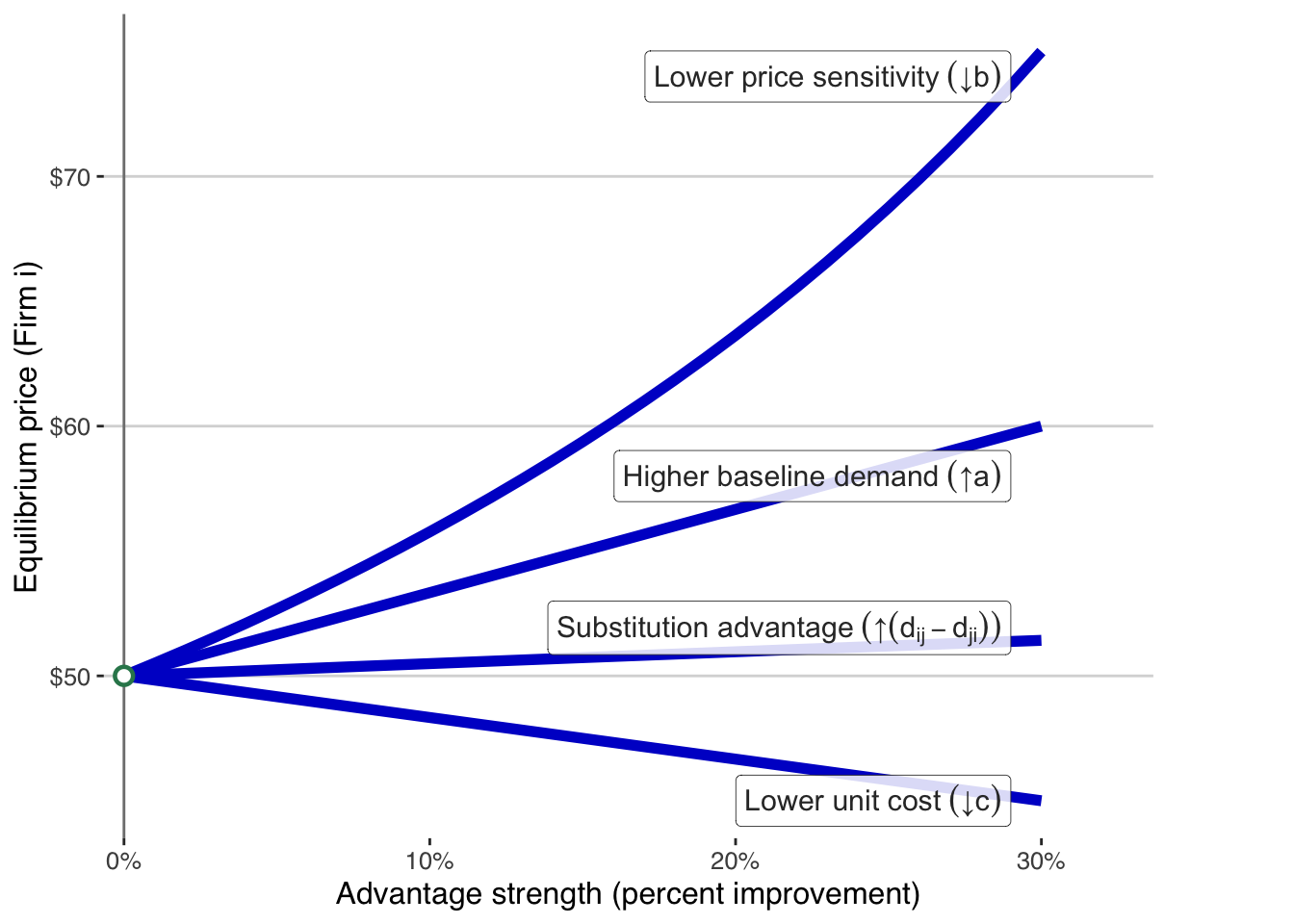
Interpreting the Structural Levers
All four lines begin at the same point.
At zero advantage, both firms are structurally identical:
- Price = $50
- Profit = $1,250
The dot marks that shared baseline.
From that point forward, each curve shows what happens when one structural lever strengthens for Firm i while everything else remains equal.
Move to the right.
Advantage increases.
Equilibrium adjusts.
1. Higher Baseline Demand (↑\(\mathsf{a}\))
When more customers value Firm i’s product at any given price, equilibrium price rises. Why? Because demand shifts outward. The firm can raise price and still retain volume.
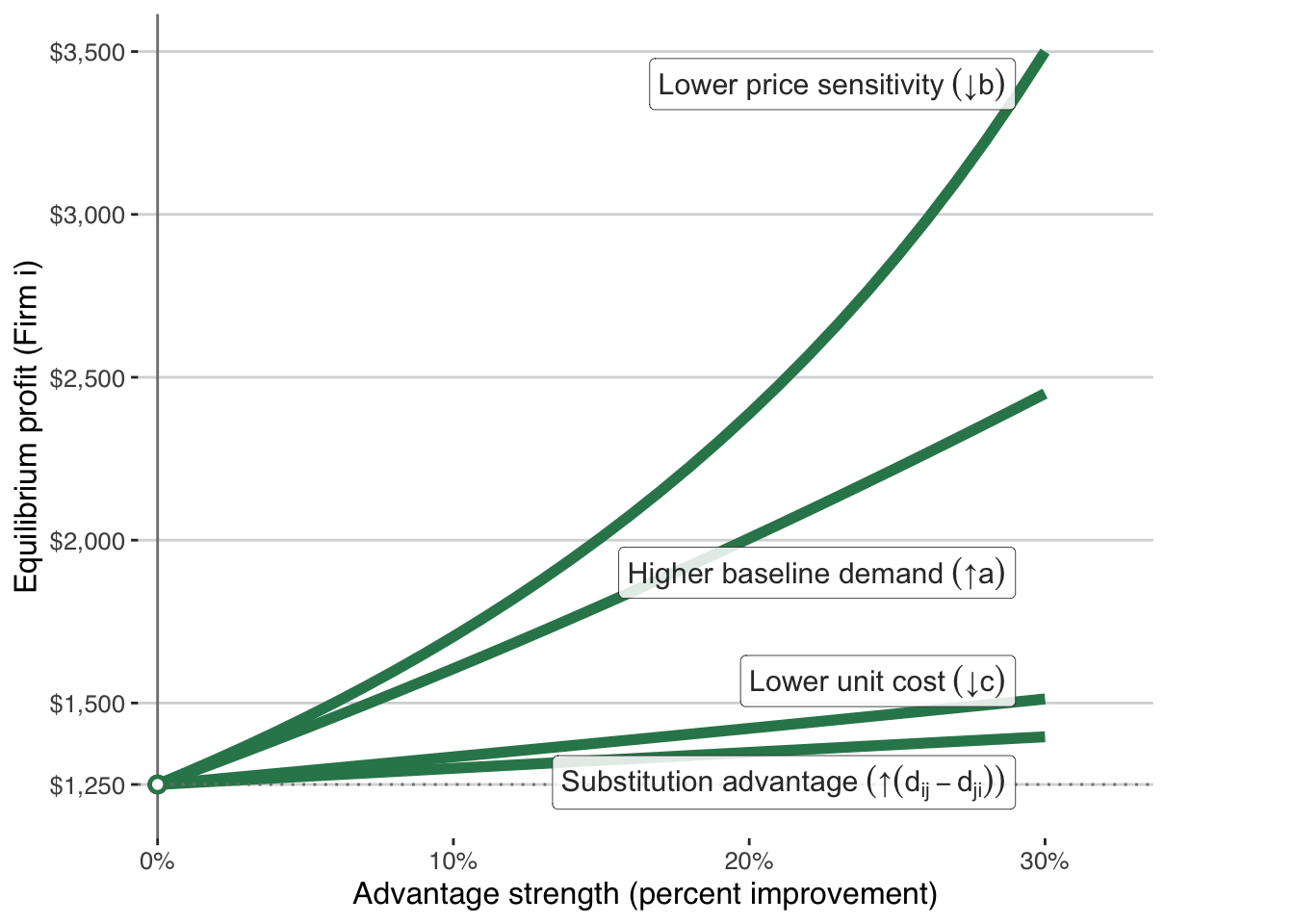
Profit increases steadily.
This lever reflects stronger overall willingness to pay — brand appeal, broader relevance, stronger perceived value.
2. Lower Price Sensitivity (↓\(\mathsf{b}\))
This is the most powerful lever in the figure.
When customers become less sensitive to Firm \(\mathsf{i}\)’s price, the firm can raise price aggressively without losing many buyers.
The price curve bends upward sharply.
Profit accelerates.
This is insulation.
It reflects design, positioning, and customer understanding.
It is rarely accidental.
3. Substitution Advantage (↑\(\mathsf{(d_{ij} − d_{ji})}\))
Here we hold total substitutability constant but tilt it in Firm \(\mathsf{i}\)’s favor.
Firm \(\mathsf{i}\) loses fewer customers when it raises price. Firm \(\mathsf{j}\) loses more customers when it raises price.
The effect is positive but moderate.
Substitution asymmetry matters — but on its own, it is not as explosive as reducing price sensitivity.
It is competitive insulation at the margin.
4. Lower Unit Cost (↓\(\mathsf{c}\))
Cost advantage moves profit directly.
Price actually falls slightly relative to baseline — because the firm optimally passes some of its efficiency into competitive positioning.
But profit rises meaningfully.
This lever works through margin, not demand.
What the Figures Reveal
Several insights become visible immediately:
- All advantages are measured relative to a common equilibrium.
- Some levers shift price dramatically.
- Some levers shift profit more than price.
- Not all “advantages” are equally powerful.
Most importantly:
Competitive advantage is not abstract.
It is parameterized.
It is measurable.
It is visible in equilibrium outcomes. It is estimated from data.
Competitive advantage is not:
- Market share,
- Revenue growth,
- Branding language,
- Or TAM slides.
It is parameter asymmetry.
When one firm enjoys stronger baseline demand, lower own-price sensitivity, weaker substitution, or lower cost, equilibrium shifts.
The strategic question becomes diagnostic:
Which parameter structurally favors you?
If none do, you do not have competitive advantage.
If one does, you can see exactly how it operates.
These structural parameters are not accidents.
They are shaped by product design, positioning, customer selection, and operational decisions.
The entrepreneur does not choose equilibrium directly — they shape the parameters that determine equilibrium.
17.4 Durable vs. Fragile Advantage
Not all parameter asymmetries produce the same kind of advantage.
Some shift equilibrium slightly.
Some shift it dramatically.
Some are easy to imitate.
Some are difficult to erode.
The figures make this visible.
When structural differences are small, equilibrium outcomes are close.
Prices differ by pennies.
Profits differ marginally.
That kind of advantage is fragile.
A small competitor response — a price cut, a minor product tweak, a modest cost improvement — can eliminate it.
Substitution and Fragility
When substitution remains high, rivalry intensifies.
Even if baseline demand differs, customers shift readily between firms when prices change.
High substitution compresses margins.
In that environment, equilibrium profit is sensitive to small parameter changes.
Advantage erodes quickly.
This is why undifferentiated markets collapse toward cost.
Discipline is severe.
Insulation and Durability
Durability appears when insulation is strong.
Lower own-price sensitivity (small \(\mathsf{b}\)) allows a firm to raise price without large quantity loss.
Asymmetric substitution (\(\mathsf{d_{ij} > d_{ji}}\)) reduces customer leakage and amplifies gains when rivals move.
When those parameters differ meaningfully, equilibrium shifts more decisively.
Price gaps widen.
Profit gaps widen.
Advantage becomes harder to neutralize.
It is embedded in the structure of demand.
Cost and Durability
Cost advantage can also be durable — but in a different way.
Lower cost increases margin directly.
It allows credible price responses.
It can discipline rivals.
But cost advantages are often more observable and more imitable than demand-side insulation.
Operational improvements spread.
Technology diffuses.
Customer insulation is frequently more persistent than process efficiency.
Structural Magnitude Matters
The key is not whether a parameter differs.
It is how much it differs.
A small reduction in \(\mathsf{b}\) produces modest shifts.
A large change in \(\mathsf{b}\) amplifies nonlinear effects in price and profit.
A slight asymmetry in substitution may be inconsequential.
A large asymmetry changes competitive equilibrium entirely.
Durability is a function of magnitude.
A Diagnostic View
Advantage is durable when:
- Parameter asymmetry is large.
- Substitution pressure is weak.
- Price sensitivity is low.
- The underlying cause of insulation is difficult to imitate.
Advantage is fragile when:
- Parameters are nearly symmetric.
- Substitution is strong.
- Customers respond quickly to price.
- The source of difference is easily copied.
Competitive advantage is therefore not a label.
It is a measurable difference in structural parameters — and its durability depends on the size and stability of that difference.
17.5 Scale and the Entrepreneurial Boundary
Competitive profit is always computed relative to a defined population.
Demand is estimated for a specific group.
Prices are chosen for that group.
Equilibrium profit is calculated for that group.
Scale enters only after structure is understood.
The Focal Population
In entrepreneurial settings, the relevant population is the one you can realistically serve.
Not the total addressable market.
Not global category sales.
Not industry revenue.
The relevant population is the defined segment for which demand was estimated.
Equilibrium profit is:
- Price × quantity,
- Within the focal market boundary,
- Given estimated demand parameters.
If you expand the population, profit scales proportionally — holding structure constant.
But expanding population does not change the structural parameters themselves.
Rival Scale
In differentiated Bertrand competition, rival scale does not directly determine equilibrium price.
Only demand parameters and cost matter.
A large incumbent may serve a broader population.
But if we are analyzing your focal segment, what matters is:
- How sensitive those customers are to price.
- How strongly they substitute.
- What your cost structure is relative to theirs.
Rival scale becomes strategically relevant only when:
- Capacity binds,
- Network effects change demand structure,
- Or multi-market interactions alter pricing incentives.
Those are extensions, not the core mechanism.
TAM Is Not Structural Advantage
Large total addressable markets can coexist with:
- High price sensitivity,
- Intense substitution,
- Thin margins.
Conversely, small segments can sustain high prices and durable profit when insulation is strong.
Scale multiplies structure.
It does not replace it.
Entrepreneurial analysis therefore proceeds in this order:
- Define the focal population.
- Estimate demand within that population.
- Compute equilibrium profit.
- Then evaluate expansion.
Structure first.
Scale second.
The Entrepreneurial Boundary
An entrepreneur’s boundary is the segment where:
- Demand is measurable,
- Cost is controllable,
- Competition is defined.
Beyond that boundary, assumptions multiply.
Within that boundary, profit can be computed.
Competitive advantage is evaluated locally before it is extrapolated globally. That discipline prevents wishful scaling.
17.6 Decision Lens
By this point, the question has changed.
In monopoly, the question was:
Is demand strong enough to sustain profit?
Under rivalry, the question becomes sharper:
Which structural parameter favors us — and is it large enough to matter?
Competitive advantage is not a story.
It is not branding language.
It is not market share.
It is parameter asymmetry.
A Structured Diagnostic
Before acting, ask:
- Is our baseline demand meaningfully higher?
- Are customers less sensitive to our price?
- Do we lose fewer customers when we raise price?
- Do we gain more customers when rivals raise price?
- Do we operate at lower variable cost?
If none of these are structurally true, equilibrium will not favor you.
If one or more are true — and large enough — equilibrium shifts.
Profit follows.
Structural vs. Temporary
A discount campaign is temporary.
A viral moment is temporary.
A short-term cost cut is temporary.
Structural advantage is embedded in:
- Estimated demand parameters,
- Relative substitution patterns,
- Cost asymmetry that competitors cannot easily replicate.
The distinction matters.
Temporary improvements shift outcomes briefly.
Structural asymmetries shift equilibrium.
The Entrepreneurial Test
The discipline of competition analytics forces a difficult but powerful question:
Is our advantage structural — or fragile?
If it is structural, equilibrium will reveal it.
If it is fragile, equilibrium will expose it.
Entrepreneurship is not the pursuit of large markets.
It is the pursuit of structural insulation within a defined market.
17.7 Where Do Structural Parameters Come From?
The parameters we have analyzed are not accidents.
They are not abstract constants imposed by the market.
They are the measurable consequences of strategic choices.
Baseline demand (\(\mathsf{a}\)) reflects how many customers value your offering at comparable prices.
Product design, positioning, distribution, and problem selection shape it.
Own-price sensitivity (\(\mathsf{b}\)) reflects how sharply customers reduce quantity when price rises.
Clarity of value, uniqueness of solution, and customer fit influence it.
Substitution intensity (\(\mathsf{d}\)) reflects how easily customers move between you and a rival.
Differentiation, targeting, and perceived similarity determine it.
Variable cost (\(\mathsf{c}\)) reflects operational design, sourcing, scale discipline, and process efficiency.
Entrepreneurs do not choose equilibrium price directly.
They shape the structural parameters that determine equilibrium.
Profit analytics does not create advantage. It reveals whether advantage is large enough to justify action.
The question of strategy becomes precise:
Have we designed the offering and chosen the segment in a way that creates structural insulation?
If the answer is no, equilibrium will expose it.
If the answer is yes, equilibrium will quantify it.
Before launch, this is the discipline.
Measure structure.
Compute equilibrium.
Then decide whether it is worth doing