8 Estimating Demand
Up to this point, the focus of this book has been on learning—how to frame the right question, design evidence that could answer it, and execute demand experiments responsibly.
At some point, however, evidence must be turned into something usable.
Decisions about pricing, investment, and scale require an object that can be reasoned about. Raw survey responses, interview notes, and scattered observations are not enough. They must be organized, structured, and interpreted.
That is the role of demand estimation.
This chapter explains what it means to estimate demand, what assumptions are being made when we do so, and how judgment enters the process. We are not teaching statistical technique here. We are clarifying what estimation is—and what it is not—so that the results can be used responsibly rather than reverently.
8.1 From Responses to a Demand Object
Estimating demand is often described as “finding” a demand curve.
This language is misleading.
Demand curves do not exist in the world waiting to be uncovered. They are not measured the way temperature or distance is measured. They are constructed—inferred from evidence using assumptions about behavior, aggregation, and continuity.
Understanding this is essential, because estimation is not a neutral mechanical step. It is an interpretive act.
What Estimation Actually Does
Before estimation, demand evidence usually looks like this:
- individual responses to willingness-to-pay questions,
- yes/no purchase intentions at specific prices,
- reported quantities tied to a period,
- variation across respondents.
None of this is yet a demand curve.
Estimation takes these scattered pieces of evidence and imposes structure on them. It answers questions like:
- How should individual responses be combined?
- How should quantity be expected to change as price changes?
- What smooth relationship best summarizes this behavior?
The result is not “the truth about demand.” It is a demand object—a structured representation that makes reasoning possible. This object allows us to:
- compare prices,
- rule out implausible scenarios,
- and connect demand to cost and profit.
But it only earns this role because of the assumptions embedded in it.
Assumptions You Are Making (Whether You Name Them or Not)
Any estimated demand curve assumes, at a minimum, that:
- customer behavior can be summarized at the market level,
- higher prices do not increase quantity demanded,
- responses vary smoothly rather than erratically,
- and unobserved prices would produce intermediate outcomes.
These assumptions are rarely stated explicitly. They are nonetheless present.
Estimation does not eliminate uncertainty. It reshapes it—turning many small unknowns into a smaller number of structured ones that can be reasoned about.
Demand estimation is powerful precisely because it is forgiving.
Given almost any dataset, a model can be fit and a curve can be drawn. That is a feature — and a risk. Before estimating anything, it is essential to verify that the data actually corresponds to a coherent demand question.
The toolkit Preparing Data for Demand Estimation provides a short set of checks to ensure that unit, period, demand type, and variation are aligned before modeling begins. Readers are strongly encouraged to work through it before proceeding.
Where the Profit Analytics App Fits—and Where It Does Not
In this book, the mechanical aspects of estimation are handled by a companion profit analytics app.
This is a deliberate choice.
Estimating demand requires computation. Interpreting an estimated demand curve requires judgment. The app exists to perform the former so that attention can remain on the latter.
The app fits demand models, compares their fit, and produces estimated demand curves from the evidence you provide. It does not decide whether the data are trustworthy, whether the assumptions are reasonable, or how much confidence the result deserves.
Those decisions remain yours.
The app will fit demand models and compare results automatically. It does not — and cannot — determine whether the data is appropriate for estimation.1
Estimation as Translation, Not Revelation
It is helpful to think of estimation as a translation step.
You begin with evidence expressed in the language of respondents: ratings, prices, quantities, intentions. Estimation translates that evidence into the language of decision-making: price–quantity relationships.
Like any translation, something is gained and something is lost.
The gain is coherence.
The loss is detail.
The purpose of this chapter is to help you understand that tradeoff—so that when you look at an estimated demand curve, you know what kind of object it is, what it summarizes, and where judgment must still be exercised.
Only then does it make sense to ask how individual responses become market demand, how different models tell different behavioral stories, and how fit should be interpreted.
That is where we turn next.
8.2 Individual Demand vs. Market Demand
Most demand evidence begins at the individual level.
A respondent states a willingness to pay.
A customer indicates whether they would buy at a given price.
A user reports how many units they would consume in a period.
These responses are real, informative, and necessary. But they are not yet the object that entrepreneurial decisions require.
Entrepreneurs do not usually price for one person.
They price for a market.
Understanding the difference—and the relationship—between individual demand and market demand is essential for using estimated demand curves responsibly.
Individual Demand Is About Preference
At the individual level, demand reflects a single person’s tradeoffs.
An individual’s willingness to pay summarizes:
- how much they value the offering,
- relative to alternatives,
- under the constraints they perceive.
This information is useful. It tells you something about appeal, variation, and heterogeneity across people.
But individual demand, on its own, does not answer questions like:
- “How many units would we sell at this price?”
- “Is demand large enough to justify entry?”
- “What price could support a profitable business?”
Those questions are inherently collective.
Market Demand Is About Aggregation
Market demand describes how quantity demanded varies with price across a population, not within a single mind.
An estimated market demand curve answers a different question:
At this price, how many units would be purchased in total by the relevant group of customers?
To answer that question, individual responses must be combined.
That combination is not automatic. It requires decisions about:
- which individuals belong in the population,
- how their responses should be weighted,
- and how variation across people translates into total quantity.
These choices are where estimation quietly intersects with sampling.
Why Representativeness Matters Here
When you estimate market demand, you are implicitly making a claim about a population.
If your sample overrepresents people who care intensely about the problem, market demand will be overstated.
If it underrepresents likely buyers, demand will be understated.
If it includes people who are not part of the target population at all, the resulting curve may be distorted in unpredictable ways.
This is why the execution choices discussed in the previous chapter matter so much at this stage.
Individual demand can be interesting even in a narrow or convenience sample.
Market demand cannot.
Once you aggregate, sampling assumptions stop being background conditions and become central to interpretation.
Why You Rarely Want “Perfect” Individual Information
It is tempting to imagine that learning demand means learning everyone’s willingness to pay precisely.
In practice, this is neither possible nor necessary.
Entrepreneurial decisions do not require knowing exactly who would buy at every price. They require knowing whether enough people would buy at plausible prices to justify action.
Market demand estimation trades individual precision for collective insight. It sacrifices detail in order to gain relevance.
This is not a weakness. It is the point.
What Estimation Adds at the Market Level
By aggregating individual responses into a market demand curve, estimation allows you to:
- reason about total quantity rather than isolated preferences,
- compare pricing scenarios at the population level,
- connect demand to costs and profit,
- and evaluate whether uncertainty is small enough to proceed responsibly.
The resulting curve does not describe any one person’s behavior perfectly. It describes a market well enough to inform a decision.
That distinction is easy to forget—and costly to ignore.
A Caution About Interpretation
Because estimated demand curves look smooth and authoritative, it is easy to treat them as objective facts.
They are not.
They are summaries of evidence filtered through:
- sampling choices,
- aggregation assumptions,
- and modeling decisions.
Used carefully, they reduce uncertainty in a disciplined way.
Used casually, they can obscure where uncertainty still lives.
The next step, then, is not to ask whether an estimated demand curve is “right,” but to ask what kind of behavioral story it tells—and whether that story makes sense for the decision at hand.
That is where model choice enters.
8.3 Choosing a Functional Form
Once individual responses have been aggregated into a sample-level demand object, another choice becomes unavoidable.
How should demand be modeled?
This is sometimes described as choosing an equation. That description is technically correct—and conceptually unhelpful.
A better way to think about model choice is this:
A demand model is a story about how customers respond to price.
Different functional forms tell different stories. The role of estimation is not to discover which story is “true,” but to identify which story is most consistent with the evidence and the decision context.
Models as Behavioral Hypotheses
Every demand model embeds assumptions about behavior.
Some assume customers respond smoothly and proportionally to price changes.
Others assume sensitivity accelerates or decelerates.
Others assume adoption saturates as price falls.
These assumptions are rarely stated explicitly, but they are always present.
Choosing a functional form is therefore not a technical detail. It is a behavioral hypothesis.
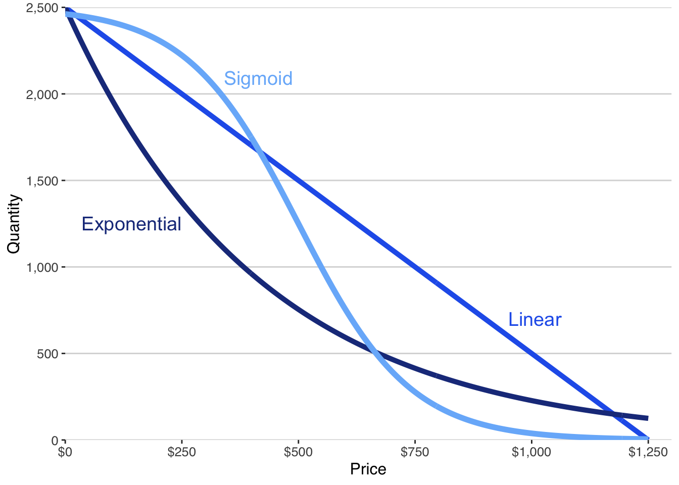
Linear Demand: Constant Sensitivity
A linear demand model assumes that quantity changes at a constant rate as price changes.
Each increase in price reduces quantity by the same amount, regardless of where you are on the curve.
This story is simple and sometimes useful, especially over narrow price ranges. But it implies behavior that is often unrealistic for new or differentiated offerings.
In particular, linear models:
- imply negative quantity at sufficiently high prices,
- and unlimited demand at sufficiently low prices.
These implications do not make the model useless. They do, however, limit how literally it should be interpreted.
Exponential Demand: Increasing Sensitivity
Exponential demand models assume that quantity responds proportionally rather than additively.
As price rises, quantity falls at an increasing rate.
As price falls, quantity grows rapidly.
This captures situations where customers become much more sensitive to price changes as prices increase—often a reasonable assumption for discretionary or substitutable products.
The behavioral story here is one of amplification: small price changes can have large effects.
As with all models, this is not a claim about truth. It is a claim about plausibility given the evidence.
Sigmoid Demand: Saturation and Adoption
Sigmoid demand models tell a different story.
They assume that:
- at very high prices, almost no one buys,
- at very low prices, almost everyone who could buy does buy,
- and most of the action happens in between.
This shape reflects two common features of real markets: - limited population size, - and diminishing returns to price cuts once adoption is widespread.
For many new products and services, this behavioral story is especially compelling. Demand grows slowly at first, accelerates as prices enter a viable range, and then saturates.
This does not make sigmoid models “better” in general. It makes them appropriate for certain kinds of decisions.
Why the App Fits Multiple Models
Because different models tell different behavioral stories, relying on a single functional form is risky.
This is why the companion analytics app estimates multiple demand models from the same evidence and allows them to be compared.
The purpose is not to select the model with the highest fit mechanically. It is to surface how sensitive conclusions are to the behavioral assumptions embedded in the model.
The app reports standard measures of fit to help you assess whether a model is consistent with the data. These measures are aids to judgment, not decision rules. A model that fits slightly worse but tells a more plausible behavioral story may be the better guide for action.
When different models tell similar stories, confidence increases.
When they diverge, judgment is required.
Model Choice Is a Judgment Call
At this point, it may be tempting to ask a simple question:
Which demand model is best?
That question sounds technical, but it is not. It is a judgment question disguised as a statistical one.
When we estimate demand, we are not uncovering a law of nature. We are choosing a functional form that imposes structure on limited evidence. Different models can often fit the same data reasonably well—and yet imply very different behavior outside the observed range.
This is why model choice cannot be automated away. It requires thinking carefully about what demand can and cannot do in the real world.
The profit analytics app estimates three common demand models:
- Linear demand, where quantity falls at a constant rate as price rises
- Exponential demand, where quantity falls proportionally as price rises
- Sigmoid demand, where demand is high and relatively insensitive at low prices, then falls rapidly over a middle range, and finally flattens near zero at high prices
Each of these models can appear plausible when viewed only through the lens of observed data. The difference lies in what they assume about customer behavior outside that data.
Why Linear and Exponential Models Often Struggle
Linear demand is attractive because it is simple and familiar. But it carries a strong and often unrealistic implication: that customers reduce quantity at the same rate no matter where price starts.
Taken literally, a linear model suggests that:
- demand can become arbitrarily large at low prices, and
- demand becomes negative at sufficiently high prices.
Both implications violate how real customers behave.
Exponential demand avoids negative quantities, but introduces a different issue. It implies that demand is always shrinking proportionally, even at very low prices. This often exaggerates sensitivity where customers are, in reality, relatively indifferent.
In practice, both linear and exponential models tend to misrepresent demand at the extremes—precisely where pricing and profit decisions are most sensitive.
Sigmoid Demand Often Fits Entrepreneurial Reality
Sigmoid demand behaves differently.
At low prices, quantity changes slowly. Customers who already value the product do not suddenly consume much more just because the price drops slightly.
At high prices, demand flattens near zero. Most customers have a reservation point beyond which they simply opt out.
Between those extremes, there is a middle region where price changes matter a great deal. This is where most real pricing decisions live.
This shape aligns naturally with how customers make tradeoffs:
- limited attention
- budget constraints
- diminishing marginal value
- and realistic saturation
The sigmoid model does not win because it fits better by default. It often wins because it respects these economic constraints without forcing them through ad hoc fixes.
Seeing the Difference
The figure below fits the same set of demand evidence with all three models.
Each model can appear reasonable over the observed price range. But as price moves beyond that range, their implications diverge sharply.
One model preserves economic plausibility across the full decision space. The others do not.
This is the heart of model choice.
Judgment Before Metrics
It is possible to rank models using statistical criteria. The app reports these diagnostics to support analysis.
But those metrics answer a different question:
Which curve passes closest to the observed points?
Entrepreneurs must answer a broader one:
Which model implies behavior that makes sense for this decision?
Model choice is not about finding the “true” demand curve. It is about choosing a structure you are willing to reason with when making irreversible commitments.
That choice cannot be delegated to a statistic.
The next section turns to a common temptation at this stage—treating good fit as proof—and explains why that move is more dangerous than it looks.
8.4 From Demand Curves to Decisions
By this point, we have done something important—but incomplete.
We have taken structured demand evidence and translated it into a demand curve. We have chosen a model that reflects how customers plausibly behave across a range of prices, not just at the points we observed.
What we have not done yet is make a decision.
This distinction matters. Estimating demand is not the goal. It is a means.
A demand curve does not tell you what to do. It tells you what could happen under different choices.
What a Demand Curve Makes Possible
Once demand is represented as a price–quantity relationship, questions that were previously vague become concrete:
- At what prices does demand meaningfully exist?
- How quickly does quantity fall as price increases?
- Where are prices clearly too low to matter?
- Where are prices clearly too high to work?
These are not optimization questions. They are questions of feasibility and plausibility.
This is why demand estimation comes before profit maximization.
Before asking “What price should we choose?” the entrepreneur must first understand which prices are even viable—and how sensitive outcomes are to that choice.
Demand curves provide that structure.
Demand Curves Do Not Choose Prices
It is tempting to think that once a demand curve is estimated, the “right” price will reveal itself.
That is not how this works.
Demand curves describe customer behavior. Prices are chosen by firms.
Choosing a price involves costs, positioning, competition, capacity, and risk tolerance. Demand estimation does not resolve these considerations. It disciplines them.
It rules out prices that cannot work and highlights regions where tradeoffs become meaningful. Within those regions, judgment still matters.
Why We Delay Profit Until Demand Is Clear
Profit depends on demand, costs, and scale. But demand is the only one of these that must be learned from customers.
Until demand is understood—even roughly—profit calculations are fragile. Small changes in assumed quantity can overwhelm careful cost modeling.
This is why this book insists on learning demand first.
Only after demand has been estimated does it make sense to layer in costs, consider fixed investments, examine competition, and reason explicitly about profit.
Demand estimation is not the end of analysis. It is the foundation.
What Comes Next
In the chapters that follow, we use estimated demand curves to reason directly about profit.
We examine how price choices translate into revenue, how costs interact with demand, and how pricing decisions emerge under uncertainty.
The profit analytics app supports this next step mechanically. The logic remains the same.
First, understand demand.
Then, reason carefully about what to do with it.
Only then does the question “Is this worth doing?” become answerable in a disciplined way.
If you have not already done so, complete the toolkit Preparing Data for Demand Estimation before using the app.↩︎