15 Differentiated Bertrand Competition
15.1 Introduction
Differentiated Bertrand competition is arguably the most prevalent form of oligopoly in real-world markets. It’s characterized by product differentiation and strategic pricing—a scenario familiar in industries like cola, desktop computers, automobiles, airlines, and ski resorts. The defining feature here, in contrast to undifferentiated Bertrand competition, is the unique characteristics of each product. To be part of this competitive landscape, the market must exhibit the following criteria:
- A Few, Influential Firms: These firms have the power to shape market equilibrium and influence their competitors’ strategies.
- Product Differentiation: Products are distinct in the eyes of consumers, who may prefer one over another based on these differences.
- Entry Barriers: These maintain the concentration of key players in the industry.
- Numerous, Individual Customers: A large customer base with limited individual market influence.
- Perfect Information: All parties are well-informed about product prices and availability.
- Price Competition: Despite product differentiation, pricing remains a crucial competitive tool.
15.2 Differentiation and the Dynamics of Pricing
Differentiated Bertrand markets allow firms to command higher, more sustainable prices, thanks to the unique appeal of their products. For instance, consider two firms offering similar but distinct products, each enjoying its own loyal customer base. A scenario where one firm offers its product for free doesn’t automatically mean the other loses all its customers. Brand loyalty and product preferences ensure that some customers remain willing to pay a premium.
In this market, firms lose the typical price war incentives seen in undifferentiated scenarios. Unique product attributes allow firms to adjust their pricing strategies flexibly. If one firm raises its price, its competitor might also increase its price, potentially adding a premium for its distinct features. This pricing interplay continues until reaching a threshold where customers no longer perceive additional value in paying a higher price.
15.3 Differentiated Bertrand Equilibrium
In differentiated Bertrand oligopolies, products are distinct yet substitutable, catering to the diverse needs of heterogeneous customers. This scenario is typical in industries where strategic pricing and product uniqueness play pivotal roles.
Demand Curves for Differentiated Products
Here, the customer’s perception of products directly influences demand. The general demand equations for two competing firms in such a market can be expressed as:
Firm 1: \(\quad \mathsf{Q_1 = a_1 + b_1 P_1 + b_{12}P_2}\)
Firm 2: \(\quad \mathsf{Q_2 = a_2 + b_2 P_2 + b_{21}P_1}\)
In these equations, \(\mathsf{Q_1}\) and \(\mathsf{Q_2}\) denote the demand for Firm 1 and Firm 2, respectively, while \(\mathsf{P_1}\) and \(\mathsf{P_2}\) are their corresponding prices. The coefficients \(\mathsf{a_1}\), \(\mathsf{b_1}\), and \(\mathsf{b_{12}}\) (and their Firm 2 counterparts) represent the demand intercept, slope, and cross-price effect, illustrating how each firm’s demand is affected by both its own and its competitor’s pricing.
Maximizing Profits with Differentiation
Profit maximization for each firm involves finding the optimal price that balances revenue and costs. The profit functions are:
Firm 1: \(\quad \mathsf{\pi_{1} = P_{1}Q_{1} - f_{1} - c_{1}Q_{1}}\)
Firm 2: \(\quad \mathsf{\pi_{2} = P_{2}Q_{2} - f_{2} - c_{2}Q_{2}}\)
Where \(\mathsf{\pi_{1}}\) and \(\mathsf{\pi_{2}}\) represent the profits, incorporating both fixed (\(\mathsf{f}\)) and variable unit costs (\(\mathsf{c}\)). Substituting the demand equations into the profit functions, we get:
Firm 1: \(\quad \mathsf{\pi_1 = P_{1}(a_{1} - b_{1}P_{1}+b_{12}P_{2}) - f_{1} - c_{1}(a_{1} - b_{1}P_{1}+b_{12}P_{2})}\).
Firm 2: \(\quad \mathsf{\pi_2 = P_{2}(a_{2} - b_{2}P_{2}+b_{21}P_{1}) - f_{2} - c_{2}(a_{2} - b_{2}P_{2}+b_{21}P_{1}) }\).
Reaction Functions
Each differentiated Bertrand oligopolist’s pricing decision is intertwined with its competitor’s pricing strategy. The relationship between the company’s optimal price and the competitor’s price is captured in reaction functions which map out the optimal pricing response to every possible competitor price.
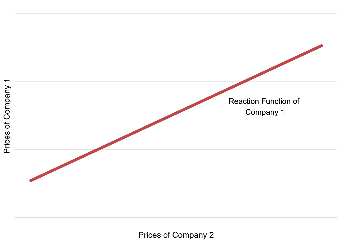
Firm 1’s Reaction: Illustrated in Fig. R1, showing how its optimal price adjusts in response to Firm 2’s pricing. Firm 2’s Reaction: Similarly, Firm 2’s optimal pricing, in response to Firm 1’s strategy, is also defined by a reaction function.
Company 1’s reaction function showing how its optimal price adjusts in response to Firm 2’s pricing is illustrated in Figure 15.1. The intercept shows that if Company 2 sets price at zero, Company 1 would still set its price above zero. The slope shows that Company 1 will optimally raise its price when Company 2 raises its price. In short, this reaction function demonstrates that each firm’s optimal price is a strategic response to its competitor’s pricing, leading to a state of mutual dependency. For Company 1, the only remaining question is “what price will Company 2 choose?”
You might already be anticipating that Company 2, much like Company 1, has its own reaction function, dependent on the pricing decisions of Company 1. This interdependence raises an intriguing question: “What price will Company 1 choose?” Logically, we are left with a strategic stalemate with both companies waiting for their competitor act so they can respond with their best price. Fortunately, there is a simple solution to the mutually dependent pricing conundrum.
Figure 15.2 introduces the reaction function of Company 2 alongside that of Company 1, providing a comprehensive view of their interactive pricing strategies. Observing Company 2’s reaction function, we notice that if Company 1 were to set its price at zero, Company 2 would still opt for a price above zero, as indicated by its reaction function’s intercept on the x-axis. Moreover, the positive slope of Company 2’s reaction function suggests a strategic response pattern: as Company 1 increases its price, Company 2 will also elevate its price proportionally.
This addition of Company 2’s reaction function to the plot not only enriches our understanding of the market dynamics but also sets the stage for identifying the equilibrium point where both companies’ strategies converge.
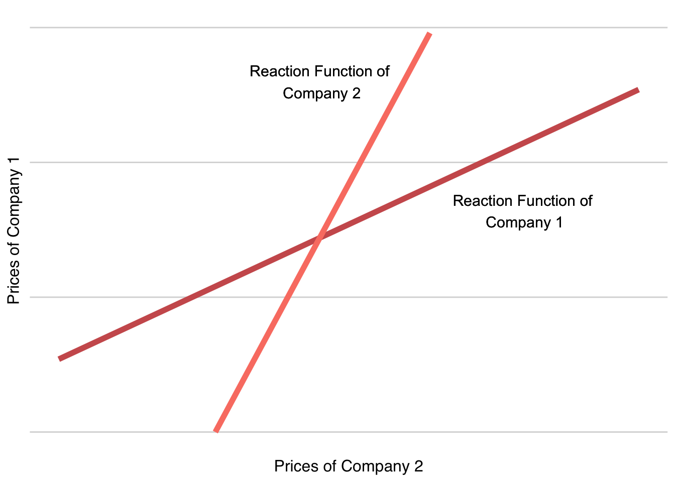
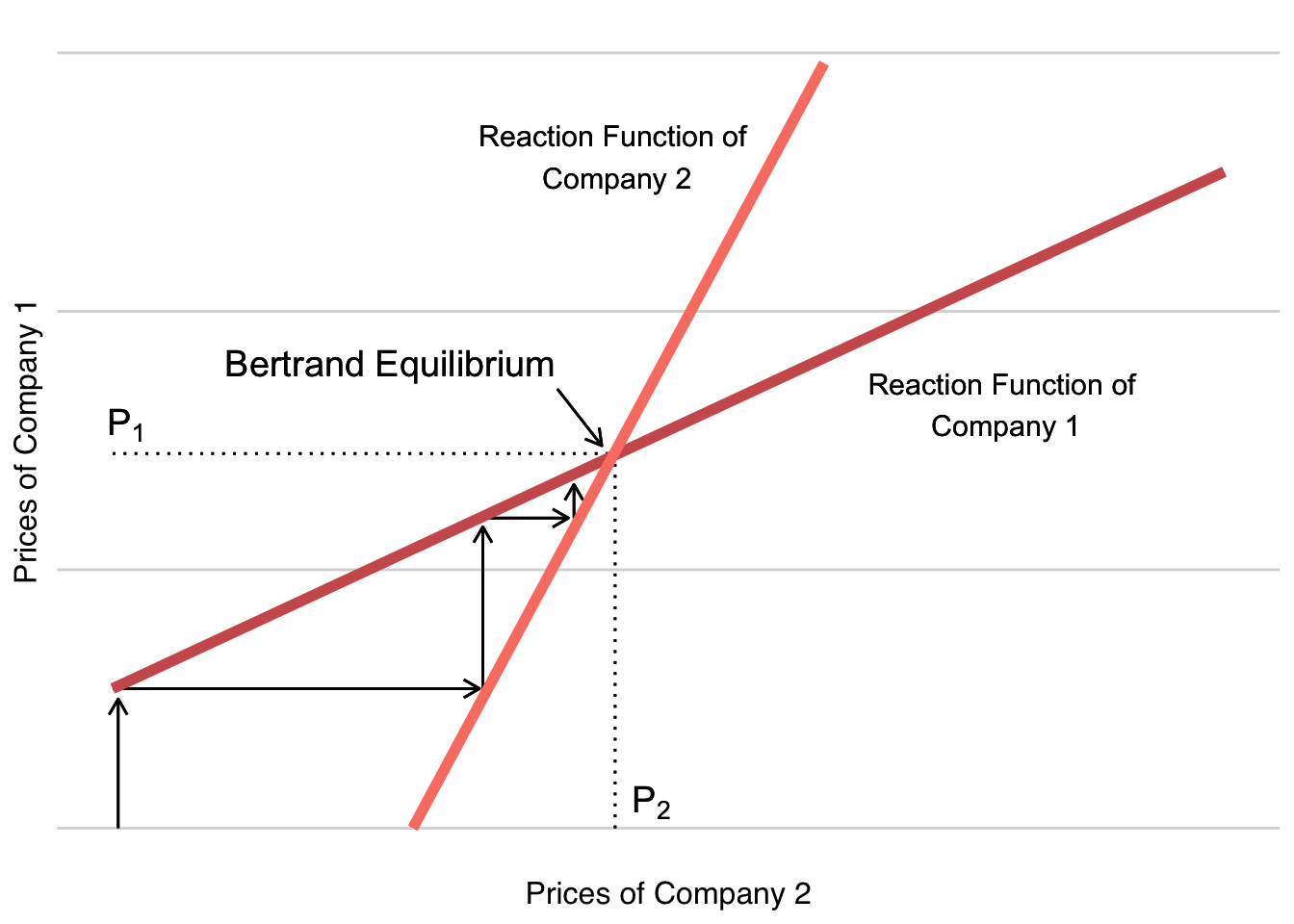
Figure 15.2 not only illustrates the individual reaction functions of Companies 1 and 2 but also reveals a critical intersection point between them. This intersection signifies where each company’s optimal pricing strategy, or best response, aligns with the other’s. In seeking to optimize, both companies naturally gravitate towards setting their prices on their reaction functions. The convergence of these functions at a single point highlights the only scenario where both firms can simultaneously choose their best responses. This point of intersection defines the optimal, equilibrium prices in our differentiated Bertrand oligopoly, as depicted in Figure 15.3.
The emergence of this equilibrium, however, raises a pertinent question: How do Bertrand competitors, without any coordination, arrive at the equilibrium prices where their reaction functions intersect? While it’s conceivable that both firms could analytically deduce and simultaneously choose the exact equilibrium prices, real-world evidence suggests this is not commonly the case.
In practice, firms often reach the Bertrand equilibrium through a process of observation and reaction. Take, for instance, Company 2 setting its initial price at zero as depicted in Figure 15.3. In response, Company 1 would set its price at the intercept of its reaction function. Company 2, observing this, adjusts its price upward to align with its reaction function, as indicated by the bottom arrow in Figure 15.3. This iterative process, characterized by a series of adjustments and counter-adjustments, eventually leads the firms to converge at the equilibrium. The key is consistent observation and responsive action, ensuring that each firm continually adjusts its pricing in line with the evolving market dynamics.
15.4 Quantitative Example: Coke v. Pepsi in Bertrand Competition
Coca-Cola and Pepsi, two of the most iconic soft drink brands, exemplify the dynamics of differentiated Bertrand competition. Utilizing demand and cost curves estimated from historical data,1 we can delve into their competitive strategies and profitability within the Bertrand framework.
Let’s designate Coca-Cola as Company \(\mathsf{c}\) and Pepsi as Company \(\mathsf{p}\). Their respective demand curves have been estimated as2
Coke’s demand curve: \(\mathsf{\quad Q_c = 63.42 - 3.98\ P_c + 2.25\ P_p}\)
Pepsi’s demand curve: \(\mathsf{\quad Q_p = 49.52 - 5.48\ P_p + 1.40\ P_c}\)
These demand curves suggest a scenario where a price increase by Coke (Company \(\mathsf{c}\)) relative to Pepsi (Company \(\mathsf{p}\)) would reduce Coke’s sales, but not all Coke consumers would switch to Pepsi. This reflects the brand loyalty found among consumers of differentiated products.
The estimated variable unit costs for Coke and Pepsi are:
Coke’s variable unit cost: \(\mathsf{\quad c_c = \$4.96}\)
Pepsi’s variable unit cost: \(\mathsf{\quad c_p = \$3.96}\)
Incorporating these costs into the demand functions, we derive the profit functions for each company:
Coke’s profit: \(\mathsf{ \quad \pi_c = (P_c - c_c) (63.42 - 3.98\ P_c + 2.25\ P_p) }\)
Pepsi’s profit: \(\mathsf{\quad \pi_p = (P_p - c_p) (49.52 - 5.48\ P_p + 1.40\ P_c)}\)
Next, we determine the reaction functions for each company:
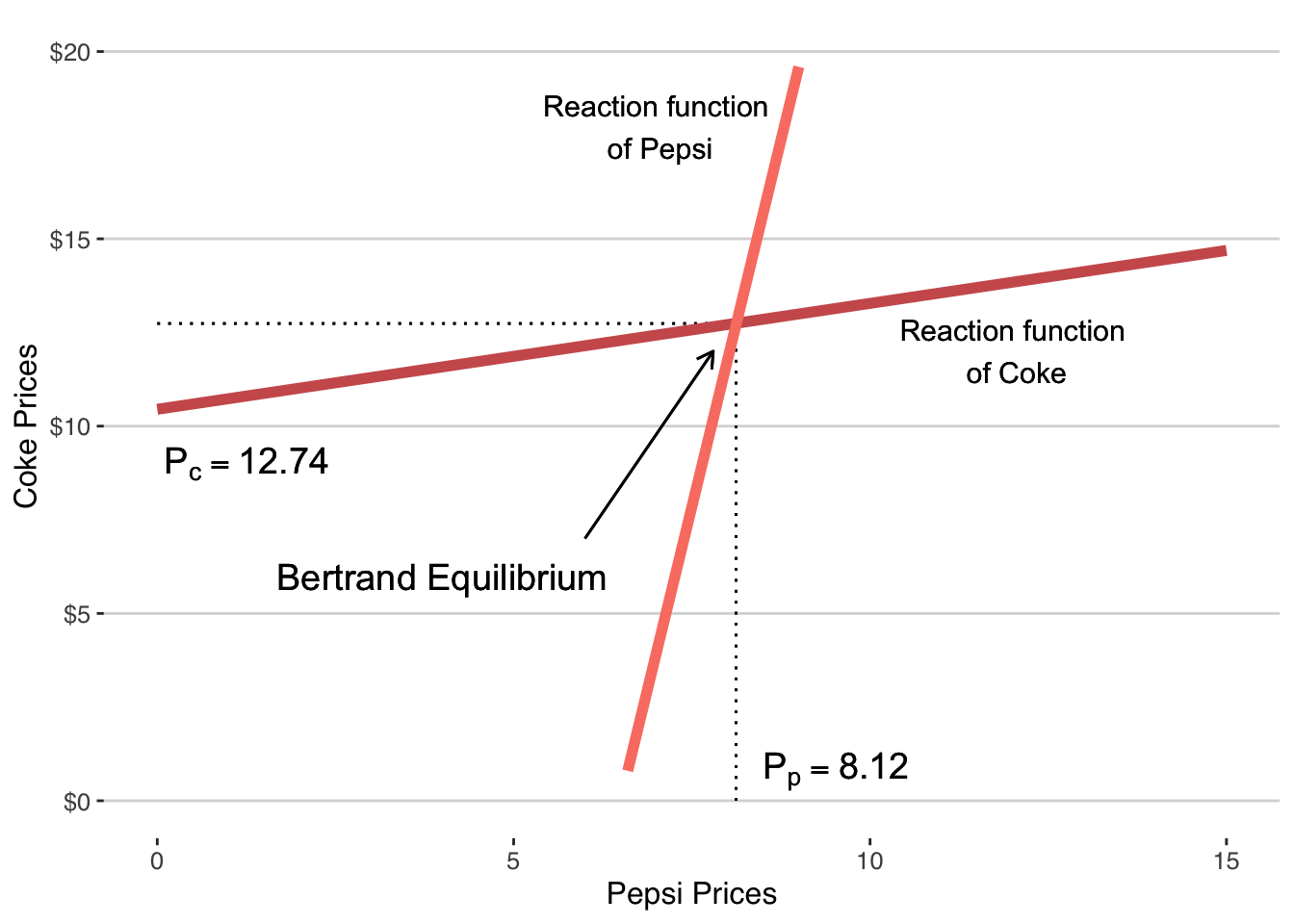
Coke’s reaction function: \(\mathsf{\quad P_c = 10.45 + 0.2827\ P_p}\)
Pepsi’s reaction function: \(\mathsf{\quad P_p = 6.498 + 0.1277\ P_c}\)
Figure 15.4 illustrates these reaction functions and the Bertrand equilibrium optimal prices for Coke and Pepsi. At this equilibrium, each company selects its optimal pricing strategy in response to the other’s pricing, balancing competitive pressure with profit maximization.
Now that we know the optimal prices for Coke and Pepsi, we can calculate their profits.
Coke’s profits: \[\begin{align} \mathsf{\pi_c} &= \mathsf{ (P_c - c_c) Q_c} \\ &= \mathsf{ (12.74 - 4.96) (63.42 - 3.98\cdot 12.74 + 2.25\cdot 8.12) }\\ &= \mathsf{\$242.71} \end{align}\]
Pepsi’s profits: \[\begin{align} \mathsf{\pi_p} &= \mathsf{ (P_p - c_p) Q_p} \\ &= \mathsf{ (8.12 - 3.96) (49.52 - 5.48\cdot 8.12 + 1.40\cdot 12.74) }\\ &= \mathsf{\$95.08} \end{align}\]
15.5 Conclusion
As we conclude our exploration of Bertrand oligopolies and their implications for entrepreneurial ventures, several critical lessons emerge. These lessons are not just theoretical musings but practical guidelines for navigating the complex landscape of market competition.
Exercise Pricing Discipline
One of the most important takeaways is the concept of pricing mutual forbearance. In the relentless quest to attract customers, the temptation to engage in aggressive price cutting can be strong. However, our analysis underscores the peril of this approach, particularly in undifferentiated markets. Instead, firms must practice restraint and avoid triggering destructive price wars that erode profitability for all players involved. Recognizing and respecting the pricing strategies of competitors can lead to a more stable and sustainable competitive environment.
The Significance of Product Differentiation
Differentiated Bertrand competition highlights the value of product differentiation and the discipline it brings to pricing strategies. Differentiation allows firms to escape the trap of competing solely on price, enabling them to command premium prices for unique product features that resonate with specific customer segments. This approach not only helps in maintaining healthy profit margins but also fosters innovation and brand loyalty.
Measure Competitiveness for Evidence-Based Decisions
Finally, the ability to compete effectively is not a matter of guesswork. It requires a rigorous measurement of expected profits and a deep understanding of one’s competitive position. In the realm of entrepreneurship, where resources are often limited and the cost of missteps high, making evidence-based decisions is crucial. By quantitatively assessing how well a venture can compete against its rivals, entrepreneurs can make informed strategic choices, from pricing to product development.
In conclusion, the journey through the nuances of Bertrand oligopolies reveals much about the strategic underpinnings of effective competition. For entrepreneurs, the lessons learned here are invaluable. They provide a framework for understanding market dynamics, a guide for strategic decision-making, and a reminder of the importance of innovation and customer focus. By applying these insights, entrepreneurs can navigate the competitive landscape with greater confidence and precision, turning challenges into opportunities for growth and success.
This equilibrium is named after the Princeton mathematician John Nash who won a Nobel prize in economics for his contributions to game theory. His journey to this discovery and eventually receiving the Nobel prize was portrayed in the film A Beautiful Mind.↩︎
Gasmi, Vuong, and Laffont (1992) used data to estimate the demand and cost curves and then analyze the Bertrand competition between the soft drink behemoths. We will reproduce their analysis here.↩︎