7 Cost Structure
7.1 Introduction
Cost is the money you pay to do the things you do to deliver value to your customers. The importance of cost is simple: if your cost exceeds your revenue, your business won’t be sustainable. Every dollar saved on costs is as valuable as an extra dollar of revenue.
Cost Structure: The cost structure is a crucial concept—it’s about how much of your costs are fixed and how much are variable. Some businesses operate with hardly any fixed costs but have higher variable cost for each unit sold. Others might have significant fixed costs, but very low costs per unit.
Your startup’s cost structure isn’t just happenstance; it’s a result of strategic decisions, much like your revenue model. The way you choose to serve your customers—a high fixed-cost model with everything in-house, or a variable-cost model relying on outsourced services—affects both your initial investment and your ongoing expenses.
Keep in mind, your chosen cost structure dictates the kind of solutions you can offer. Not all cost structures can support the same solutions, and the most effective solution isn’t always the most cost-effective one.
Selecting a cost structure is as fundamental as choosing how and when to invest in the resources that will become your fixed costs. Understanding the nature of your costs is the first step towards making informed decisions about your business’s financial future.
7.2 The Nature of Cost
Costs are the sum of all expenses a business incurs to produce and deliver its services or products, encompassing everything from labor to utilities. These costs define how a business allocates its resources and sets prices.
Total Cost
Total cost reflects the entire expense of producing a given level of output in a period of time. It’s critical to understand that while historical data often inform cost analyses in existing companies, entrepreneurs must instead estimate future costs to make informed decisions. Without historical data to rely on, we typically forecast a linear approximation of total costs, such as
\[\begin{align} \mathsf{C} &= \mathsf{cQ + f} \\ &= \mathsf{50\,000 + 200\ Q} \end{align}\]
where \(\mathsf{C}\) is total cost, \(\mathsf{c}\) is the variable cost per unit, \(\mathsf{f}\) is the fixed cost and \(\mathsf{cQ}\) is the total variable cost.
Before revenue, you will typically have complete knowledge of your future variable and fixed costs. As your business evolves and you gather actual data, these cost functions can be refined.
Understanding the composition of total costs is foundational. Fixed costs, like rent, remain constant regardless of output levels. Variable costs, such as materials and labor, fluctuate with production volume. The interplay of these costs dictates pricing strategies and potential profit margins.
The relationship between fixed and variable costs, and their total, is illustrated in Figure 7.1, where the fixed cost is \(\mathsf{ f = 50\, 000}\) and the variable cost per unit \(\mathsf{c = 200}\) is the rate at which total cost rises as quantity increases.
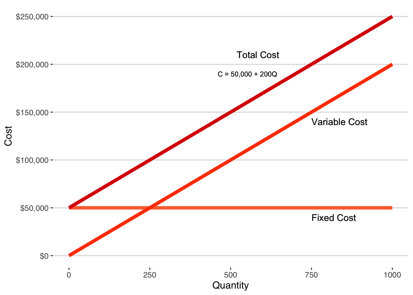
Entrepreneurs must navigate these concepts with both foresight and flexibility to build a sustainable cost structure for their ventures.
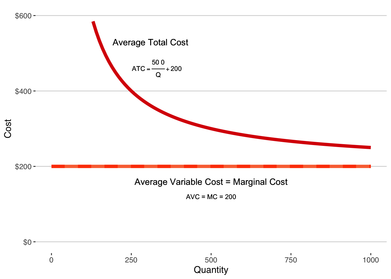
Unit Costs
Understanding unit costs is imperative for businesses to ensure they price their products or services appropriately. It’s not merely about covering total costs but also ensuring each unit sold contributes to the overall financial health of the business. Unit costs, also known as “cost per unit,” refer to the cost incurred by a company to produce, store, and sell one unit of a particular product or service. This measure is crucial for businesses to calculate in order to set appropriate selling prices, determine break-even points, and strategize for profitability. Unit costs can be broken down into various components, such as:
Average Total Cost (ATC)
This is the total cost of production divided by the number of units produced. It encompasses all costs, both fixed and variable, averaged over all units of output. The formula for ATC is:
\[\begin{align} \mathsf{ATC} &= \mathsf{\dfrac{C}{Q}} \\[9pt] &= \mathsf{\dfrac{f + cQ}{Q}} \\[9pt] &= \mathsf{\dfrac{50\, 000 + 200Q}{Q}} \\[9pt] &= \mathsf{\dfrac{50\, 000}{Q} + 200} \end{align}\]
We can see that average total cost ATC comprises average fixed cost and average variable cost.
If the chosen price of a product is below the ATC, it may be unsustainable to enter the market or continue operations. The equation for ATC often highlights the benefits of economies of scale – as production increases, the fixed cost contribution per unit decreases, potentially lowering the ATC.
Average Variable Cost
Average variable cost (AVC) specifically looks at the costs that vary with production. Keeping prices above AVC is crucial in the short run to ensure a business isn’t operating at a loss. This measure helps in making incremental production decisions, especially when considering the minimum price at which it’s viable to keep producing.
\[\begin{align} \mathsf{AVC} &= \mathsf{\dfrac{VC}{Q}} \\[9pt] &= \mathsf{\dfrac{cQ}{Q} = c} \\[9pt] &= \mathsf{\dfrac{200Q}{Q} = 200} \end{align}\]
Marginal Cost
Marginal cost (MC) represents the cost of producing one additional unit. In a linear cost model, the marginal cost is constant and identical to average variable cost, simplifying decision-making. It’s vital for making informed decisions about increasing or decreasing production levels and for setting competitive prices.
These unit cost measures are visually represented in Figure 7.2, allowing for a clearer understanding of the cost implications at different production levels.
Time and Cost: The Short-Run vs. The Long-Run
The perspective on what constitutes a fixed or a variable cost can shift based on the time frame considered. In the short run, certain costs are fixed because the firm’s scale of operations cannot be adjusted quickly— for example, the rent for a factory. In the long run, as the firm has the opportunity to adjust its scale of operations, these costs become variable.
Thus, the categorization of costs as fixed or variable is less about the nature of the cost itself and more about the firm’s ability to modify these costs within a given time frame. This time sensitivity is crucial in strategic planning, as it influences the flexibility of a business to adapt to market changes and manage its cost structure for sustainable growth.
Fixed costs vs. Sunk Costs
Fixed costs and sunk costs are often conflated but they have differences that are important in making decisions about investments in infrastructure that increases fixed costs. Here’s a detailed look at the differences between the two and how they relate to decision-making:
Fixed Costs
Fixed costs are business expenses that remain unchanged regardless of the level of production or sales. These costs are “fixed” over a specified period and do not fluctuate with the volume of output. Examples include rent, salaries of permanent employees, depreciation of machinery, and insurance. These are costs a company incurs just for being in business, whether it produces anything or not.
Fixed costs can sometimes be altered or eliminated, but this usually requires a strategic shift or long-term planning. For example, a company might relocate to a cheaper facility or downsize its staff to reduce its fixed costs.
Sunk Costs
Sunk costs, on the other hand, are costs that have already been incurred and cannot be recovered. They are “sunk” because they are past expenditures that can no longer be affected by current or future actions. For instance, if a company invests in research and development for a product that it later decides not to produce, the money spent on R&D is a sunk cost.
Sunk costs should not influence future business decisions since they cannot be recovered or changed. However, businesses and individuals often fall prey to the “sunk cost fallacy,” where they continue investing in a project due to the amount already spent, rather than based on future viability.
Decision-Making and Cost
In decision-making, particularly within economics, it’s essential to focus on relevant costs which include opportunity costs and incremental costs. Opportunity costs represent the benefits a business misses out on when choosing one alternative over another. Incremental costs are the additional costs incurred when making business decisions, such as producing additional units.
Opportunity Cost: This is the cost of the next best alternative that is foregone when a decision is made. It’s the value of what you could have done versus what you actually chose to do.
Incremental Cost: When comparing options, it’s the additional cost over the current expenditure. It’s crucial for decision-makers to consider incremental costs rather than sunk costs because they reflect the potential future impact of decisions.
Accounting vs. Economic Perspective
Accounting: From an accounting standpoint, sunk costs are recognized and cannot typically be adjusted. They are recorded as they are incurred and may affect overall profitability.
Finance: In finance, particularly when conducting cash flow analysis, the timing of cost recovery is crucial. Fixed costs that can be recovered, such as through the sale of an asset, are considered when calculating the net present value or internal rate of return.
Economics: Economists consider only those costs that can affect future decisions. Sunk costs are irrelevant to future economic decision-making because they do not change regardless of the outcome of future events.
Understanding the difference between fixed and sunk costs is vital in making informed decisions that affect the economic health of a company. Decision-makers must look beyond past investments (sunk costs) and focus on the costs and benefits that can be influenced by their decisions (incremental and opportunity costs).
Cost Structure and the Business Model
Let’s explore the relationship between cost structure and the business model. We choose both the cost structure and the business model and both need to be taken into account because different business models inherently have different cost implications:
Production Revenue Model
Variable Costs: These include costs that vary with production volume such as raw materials, inventory costs, piece-rate labor (wages paid per unit produced), and sales commissions that are tied directly to the number of units sold.
Fixed Costs: Costs that remain constant regardless of production volume, such as salaries for management, costs related to the manufacturing facility, equipment, and general overhead.
Retail Revenue Model
Variable Costs: In a retail environment, the variable costs mainly consist of the cost of goods sold (purchases of inventory that will be resold) and sales commissions if applicable.
Fixed Costs: The costs of operating a retail space (rent, utilities, etc.), purchasing staff salaries, and general overhead expenses remain fixed.
Licensing Revenue Model
Variable Costs: For a licensing model, the costs that vary with the number of licenses sold could include sales commissions and legal costs for drafting and enforcing contracts.
Fixed Costs: The substantial investments in research and development (R&D) to create the intellectual property (IP), and the legal costs associated with securing IP rights (patents, copyrights, trademarks).
Scalability Challenges
Labor-Intensive Solutions: Businesses that rely heavily on human labor (like consulting or teaching) are less scalable because costs increase linearly with revenue. To grow, you need to hire more people, and profit margins don’t significantly improve due to the proportional increase in labor costs.
Asset-Intensive Solutions: For businesses that require physical assets like property or buildings, scaling up often means acquiring more assets, which leads to a proportional increase in costs relative to revenues.
Cost Structure and Profitability
Scalability and Margins: The ideal business model is one where costs do not grow at the same pace as revenues, allowing profit margins to increase with scale. Web-based solutions are a prime example, as they require minimal additional costs for serving additional customers, thus scaling effectively.
Trade-off Between Fixed and Variable Costs: Investing in scalable fixed assets can often reduce variable costs and allow for better scalability. However, such fixed costs can be significant and challenging for entrepreneurs to fund, especially in the early stages of a startup.
Entrepreneurial Challenges
For entrepreneurs, particularly in the startup phase, there is often a tension between the desire to invest in scalable assets and the reality of limited funds. This often results in a reliance on higher variable costs due to a lack of capital to invest in fixed, scalable assets. Entrepreneurs must navigate this trade-off while seeking funding sources that can support investments in assets that will help them scale more effectively in the long run.
In essence, the choice of business model and the resulting cost structure are crucial in determining how easily a business can scale and how its profitability will change as it grows.
7.3 Where Do We Get Cost Curves?
For Established Firms:
- Established firms often have a well-documented history of their input usage, allowing them to derive accurate cost curves.
- Some companies go to lengths such as hiring consultants to estimate competitors’ cost functions, which can involve indirect methods like monitoring deliveries.
For New Ventures:
- New ventures face uncertainty regarding the cost of inputs since they lack historical data.
- Early cost estimates must be made without complete knowledge, which is risky and potentially inaccurate.
- Costs can be influenced by factors like purchase volume and supplier relationships, making initial estimates challenging.
- Entrepreneurs sometimes erroneously assume that knowing the cost of goods sold equates to understanding their entire cost structure.
Gathering Cost Information
Physical Products:
- Use market prices for standard materials.
- Obtain tentative quotes for customized inputs.
Software/Services:
- Base estimates on local labor rates for established job functions.
- For specialized roles, discussions or negotiations with potential workers may be necessary.
Cost Efficiency:
- The subsection cautions that the assumption of efficient input usage might not hold true in practice.
- Inefficiencies, like congestion during a move with too many helpers, can lead to higher costs than necessary.
- Overcoming these inefficiencies requires targeted efforts to optimize production and service processes.
7.4 Choosing a Cost Structure
Early Stages
Bootstrapping Phase: Startups often begin with minimal fixed costs; operating out of a free space and covering expenses via personal means, maintaining flexibility by using external services.
Cost Minimization: The goal is to keep fixed costs low until there is proof of demand for the product, thus avoiding unnecessary financial burdens.
Growth and Scaling
Initial Growth: As the product gains market traction or investment is secured, the startup can afford to incur more fixed costs like office space and salaries.
Hiring Key Talent: Skilled professionals are brought on board to refine and build the product.
Founder Compensation: Founders may start with modest salaries, their main compensation being the growing value of their equity.
Maturation
Established Presence: A successful venture with significant market share may invest in permanent assets, such as buildings, and start developing a more hierarchical structure.
Professional Management: The operational complexity may lead to the hiring of professional executives to manage the company’s growth and operations effectively.
Cost Structure Transition
The decision to shift from a lower fixed cost structure to a higher one depends on the company’s scale and its ability to cover fixed costs. Figure 7.3 shows how total costs vary with different ratios of fixed to variable costs, illustrating the optimal points for transitioning.
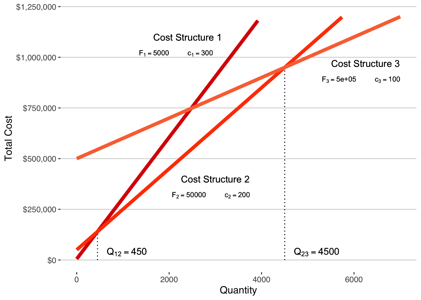
Strategic Decisions
- Avoid Premature Fixed Costs: Entrepreneurs should resist investing in large fixed assets too early, as customer needs and solutions are still evolving.
- Incremental Investments: It is advisable to gradually improve the product with a focus on adaptability, even if that means higher variable costs initially.
Considerations for Startups
- Startups should carefully assess when to transition to a cost structure with higher fixed costs.
- The goal is to minimize costs at the current level of scale, avoiding the trap of scaling fixed costs too quickly which could lead to unprofitability.
- The timing of these transitions is critical and can be guided by analyzing cost curves and scale of operations.
This provides a strategic framework for startups to consider when scaling their operations, emphasizing the importance of aligning cost structures with stages of growth and the inherent risks of moving too quickly into high fixed costs without the sales volume to support them. It is a crucial guide for entrepreneurs to understand the financial implications of growth and scale in the context of a startup lifecycle.
The Decision to Make or to Buy
The make-or-buy decision shapes your startup’s cost structure at a fundamental level. Producing goods in-house generally ramps up fixed costs due to the need for equipment, space, and expertise. On the other hand, procuring goods from a supplier increases variable costs, as you pay for their production plus a margin.
Conventional wisdom advocates for startups to purchase inputs, conserving resources to innovate on what can’t be bought. The challenge lies in discerning when it’s financially wiser to produce rather than purchase.
Purchasing inputs can shift substantial fixed costs to the supplier, leaving your startup with higher variable costs. However, the total purchase cost may exceed in-house production if the supplier’s profit margin is steep. Alternatively, a supplier’s specialized operations can result in lower costs for you, even with their profit margin included.
Transaction Costs
When buying, consider transaction costs—the risk and governance expenses in transactions (Williamson 1975, 1985). Suppliers can falter, causing holdups that delay your operations. Contracts and strong relationships are governance mechanisms that reduce such risks, but in cases of significant holdup risk, in-house production might safeguard your startup’s future.
Entrepreneurial decisions should weigh these transaction costs. For low-risk inputs, buying is typically safe. For high-risk inputs, manufacturing internally may be essential. Refer to Section 7.7 (Appendix A) for an in-depth analysis of transaction cost economics and the make-or-buy conundrum.
7.5 References
7.6 Workout Problems
Cost structure of the Dorsal travel pack
The Dorsal travel pack is a stylish, modern backpack with all of the zippers facing inward toward the wearer’s back. It is made of slash resistant fabric in nondescript colors to avoid the attention that more popular colorful brands draw. Let’s look at the cost of having the Dorsal pack manufactured by a contract manufacturer. The manufacturer charges $40 per backpack to be manufactured, packaged, and delivered to the start-up’s offices. The start up is also spending $200 per month for web hosting and $5500 per month for contracted web development. Their total cost curve is linear: \[ \mathsf{C = cQ + f}\] where \(\mathsf{c}\) is the variable cost per unit and \(\mathsf{f}\) is fixed cost per month.
In homework 2, we studied revenue models for the Dorsal travel pack. In this homework, we will continue the analysis by focusing on cost of the backpack.
What is the variable cost per unit for the Dorsal pack?
What is the average variable cost of producing and selling 32 Dorsal packs?
What is the fixed cost per month?
What is the total cost of the first 62 units?
What is the total variable cost of 37 units?
What is the total fixed cost of 75 units?
What is average total cost of 43 units?
Investing in new cost structure: Like most start-ups in the early days, Dorsal pack has embraced a cost structure with low fixed costs and high variable costs. In the next stage of business model development, they are considering doing the packaging and order fulfillment themselves. In this scenario, the manufacturer would ship to the finished product in bulk to Dorsal’s headquarters. Without packaging, the manufacturing cost is $25. A single person can manage the packaging and order fulfillment operation once it is set up. The cost of setting up packaging and fulfillment operations is $16,000 per month. This cost is in addition to the fixed costs from original cost structure that will remain in the new cost structure. How many travel packs does Dorsal need to sell per month to justify moving to the new cost structure by investing in packaging and fulfillment?
Note that you can use a ggplot with a layer for each function (using geom_function twice) to roughly find the point where two functions intersect. However, to know the precise value where intersection happens, you first create a new function that is the difference between the functions (f1intersect2 <- function(x) f1(x) - f2(x)). Then use the packagerootsolve(you will probably need to install it) to find the roots of the new function. When the difference between the functions is equal to zero, they have intersected one another. The syntax for usingrootsolveisuniroot(f1m2, lower = #, upper = #)wherelower =andupper =provide the values of \(\mathsf{x}\) that are the lower bound and upper bound to search for the intersection.The impact of pricing on cost:. We have been working with cost as a function of quantity which is traditional. However, we will normally make the pricing decision to tell us what the quantity demanded will be. To incorporate price into decisions about cost, just insert the demand curve \(\mathsf{Q(P)}\) in place of the quantity variable in the cost equations. In the case of the Dorsal travel pack, we estimated the demand curve in Homework 1 and 2 to be \(\mathsf{Q_{dp} = e^{5.115604 - 0.011612\cdot P}}\).
- Using this demand curve, what is the expected total cost when we set the price at $100?
- What is the average total cost when the price of a dorsal pack is $200?
- Using this demand curve, what is the expected total cost when we set the price at $100?
7.7 Appendix A: Clarifying the Make-Buy Decision through Transaction Cost Economics
A common question that entrepreneurs face is whether to make a particular input to their solution or to buy it from a supplier. For example, a startup with a software-as-a-service (SAAS) solution needs a great deal of computing capacity to serve the customer needs that come from around the globe. Should the startup buy, host, and maintain its own web servers or should it contract with one of the many cloud computing providers? For a SAAS startup, the wisdom of ``buying everything you can’’ means that a contract provider of cloud computing should be used. When you consider the costs and hassles of buying, installing, maintaining, and securing the computers, it sounds logical to let the experts focus on their strength in computer hardware while the startup focuses on its expertise in building a software solution.
Much like the concept of opportunity cost, transaction costs often do not show up in the direct and indirect accounting costs of making and delivering your solution. As a result, it is easy to neglect or ignore the influence of transaction costs in your decisions. When transaction costs are large, ignoring them can lead to decisions that are very costly and even fatal to your company.
The risk of holdup demands governance mechanisms to facilitate transactions. Let’s first explore the factors that lead to the risk of holdup: uncertainty, bounded rationality, opportunism, and asset specificity. When there is certainty about a transaction or the markets of the supplier and the buyer, there is no risk of opportunism. If you are certain about what will happen, there will be no surprises and you will only transact if it is safe.
When there is uncertainty, surprises happen. When there is uncertainty, it is not possible to write a fully contingent contract–one where every possible contingency is addressed and agreed upon—so the unexpected can happen to either or both of the transactors. Surprises often lead to unexpected problems that make it impossible to fulfill the terms of the contract and holdup happens. Uncertainty causes the parties to a transaction to have bounded rationality meaning that their ability to foresee and specify risks is limited. Since we all have limits to our rationality, especially in our ability to see through uncertainty, you must evaluate the risk of holdup in our transactions.
Some suppliers are more trustworthy than others. Usually, you perceive that a supplier is less trustworthy because they show a tendency or a history of opportunism. Opportunism is a willingness to take advantage of the other party in a transaction, even resorting to guile to take advantage and get ahead. It is not necessary for every possible transactor to be opportunistic. It is not even necessary for one of the transactors of a particular transaction to be opportunistic. If there is uncertainty and you can not be sure that the other transactor is honest, the risk of opportunism is present and you must respond to it.
Some inputs to your solution will be generic type inputs for which there are many competing suppliers competing in commodity markets to sell to you. Other inputs are specific to the transaction and open the door to holdup. A specific asset is one that cannot be redeployed to new uses if the transaction fails. The inability to redeploy the asset means that it is closely related to the sunk costs we discussed in Section 7.2.4.
To see the relationship between asset specificity and the risk of holdup, consider the case of injection molding. Injection molding, as the name suggests, injects a material into a mold to quickly produce a physical part in a desired shape. The mold must be created to exacting standards to produce the desired shape of the finished part. As a result, it can almost never be used in another application. We would say that the mold is an asset that is specific to the transaction for that particular molded part. The high degree of asset-specificity of the mold is the primary source of the risk of holdup. Once the molding company has incurred the cost of creating the mold, that cost is sunk. The buyer can come back to the supplier and demand a price reduction. Since the cost of the mold is sunk, the supplier has little leverage and will likely have to give in.
When assets are highly specific to the transaction and the risk of opportunism is high, the transaction costs may be so high that transactions never happen. In practice, transactions between customers and suppliers of injection molding because the customer is required to buy the molds.
Transaction cost economics identifies at least six types of asset specificity that raise the risk of holdup:
Site Specificity: when a supplier locates production near a buyer, or vice versa, for the sake of lower transportation costs and increased coordination, the cost of relocating and the cost of changing suppliers increases;
Physical Asset Specificity: when a physical asset can only do one thing for one buyer, it cannot be redeployed and the risk of holdup increases;
Human Asset Specificity: when employees develop knowledge and skills that can only be used in a particular employer, the cost of the employee leaving is higher for both the employee and the firm;
Temporal Specificity: when there is a window of opportunity after which value is lost such as in earning an on-time delivery bonus or earning a first-mover advantage, buyers are vulnerable to suppliers who are slow to deliver;
Dedicated Assets: when a customer invests in assets for a particular supplier or when a supplier invests in assets for a particular customer, the cost of redeploying the may be very high if it is even possible;
Brand-name Capital: brand equity is tied to the firm that developed it and is difficult to transfer to another firm or brand. It is harder to build brand equity than to sustain it so firms with brand equity are vulnerable to firms who can damage it without damaging their own brand.
The risk of holdup threatens to derail transactions when the risk is particularly high. The solution is to implement a governance mechanism that reduces the risk of holdup to levels that allow transactions to proceed. We saw an example of a governance mechanism in the transactions for injection molding. The supplier requires the buyer to pay for the mold before the mold is built. Because the buyer bears the fixed cost, the primary opportunity for the buyer’s opportunism is eliminated. This particular governance mechanism is known as where the giving of a hostage (the molds) aligns the incentives of the buyer and the supplier and allows them to transact with confidence.
There are three primary categories of governance mechanisms with varying effectiveness in eliminating holdup cost. The first category is the spot market which is sometimes known as “cash and carry.” For example, if you need paper for your printer, you typically go to a retailer, give them cash, and carry away the paper. This governance mechanism is weakest in terms of reducing the risk of holdup but it is also the cheapest and easiest to implement. When the risk of holdup is low enough, it works well.
At the other extreme of the governance mechanism continuum is hierarchy which means that the transaction happens inside the hierarchy of the company. Hierarchy is a very powerful governance mechanism because even when there is high asset specificity, the risk of holdup is low. If one division of a company exercises opportunism against another division of the same company, the opportunistic division may be better off but the company is injured overall. An executive of the company can rein in the opportunistic division, sort out the differences and ensure a collective benefit for the company. The downside of hierarchy is that it is expensive. A new division of the company has to be formed; new employees and managers must be brought in and trained; new executives and executive responsibilities must be adopted; and coordination between divisions grows geometrically as the number of divisions grows.
Between the extremes of market and hierarchy is the hybrid category which contains elements of market and hierarchy. The simplest hybrid form is a contract that defines how the buyer and the seller will act under various contingencies. A contract is more effective than the spot market in overcoming the risk of holdup but it is more expensive in terms of contracting costs and coordination. A contract is less effective than hierarchy in overcoming holdup because courts must be used to resolve disputes but it is cheaper to set up and coordinate. Alliances, joint ventures, and franchises are additional forms of hybrid governance mechanisms. Each is closer to hierarchy than contracts and more effective in reducing holdup but also more expensive.
While governance mechanisms are effective in reducing or eliminating the risk of holdup, their cost must be included in the total transaction cost. The total transaction cost is the sum of the cost of the governance mechanism and the cost of the remaining risk of holdup. The varying governance mechanisms have varying costs. In general, more effective governance mechanisms are also more expensive to implement and are only cost effective when the risk of holdup is high such as when there is high asset specificity. This insight is illustrated in Figure 7.4, adapted from Oliver Williamson (1985), where we see the cost of the governance mechanism graphed against the degree of asset specificity which directly causes the risk of holdup.
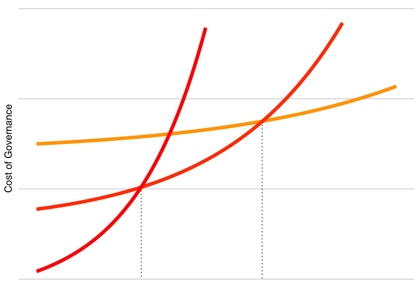
When asset specificity is low, spot market governance works well and has a low cost. However, as asset specificity grows, the cost of governance using spot markets grows much faster due to the cost of monitoring, coordinating, and the cost of holdup. When there is no asset specificity, the hybrid governance mechanism has a higher cost than markets because of the cost of setting up legal contracts and coordination. With very low asset specificity, hybrid governance is a poor choice. As asset specificity rises, the cost of governance rises and eventually hybrid governance becomes the least expensive choice for moderate levels of asset specificity. In the absence of asset specificity, hierarchy is the most expensive governance mechanism. As asset specificity rises, the cost of governance rises more slowly so that hierarchy is the least expensive choice for high levels of asset specificity. The choice of appropriate governance mechanism is straightforward. Choose the mechanism that minimizes the transaction costs given the level of asset specificity.
What does this mean for the entrepreneur? The debate over which inputs to make and which to buy is best resolved through the lens of transaction cost economics. The traditional wisdom is that entrepreneurs should buy every input they can. This is good advice for inputs with low asset specificity where spot markets can be used and for inputs with moderate asset specificity where contracts or partnerships can be used. In contrast, when asset specificity for a transaction for an input is high and the risk of holdup is also high, you are better off to make that input. Even when it is available to be purchased in the market, the risk of holdup is so high that the well-being of your startup is in jeopardy when you buy the input rather than make it.
7.8 Appendix B: Economies and Diseconomies of Scale
There are diverse reasons why average total cost falls as scale increases. The primary reason is the spreading of fixed costs over more units sold. On top of that, economies of scale may result from increased efficiency as scale increases.
Economies of Scale
Product-Specific Economies of Scale
These economies of scale are associated with the volume of a single product.
At higher volumes, specialized investments in machines and human capital (both R&D and production) allow for production methods that reduce the cost per unit. In particular, labor costs decrease due to increases in proficiency as well as fewer errors per unit. For example, in ball bearing manufacturing, production of less than 100 rings is done by hand on general purpose lathes. For production between 100 – 1,000,000 rings, production is done with a specialized screw machine. For production greater than 1,000,000 rings, production is done with an even more specialized high speed, continuous process machine.
Increased bargaining power in procuring raw materials/inputs decreases the cost of raw material inputs.
Plant-Specific Economies of Scale
These economies of scale are associated with the total output of an entire plant.
- Efficiency gains that result from expanding the size of individual processing units and sharing plant costs across several related products (e.g., procurement, inventory management/receiving, transportation/distribution). These types of efficiency gains are
- Energy usage — rises less than proportionately with increases in processing size.
- Labor — crews required to operate a large processing unit or machine are often no larger than what is needed for a unit with smaller capacity.
- Massed reserves — lower costs for back-up of specialized machines (e.g. you need a back-up if you have one or five machines running). Fewer maintenance personnel are required per machine/plant; also useful when unit/machine shutdowns occur regularly and predictably.
Economies of Multi-Plant Operations
These economies of scale are associated with total corporate size.
- Economies of scale in centralized service functions, such as R&D and management/staff. Costs per unit are lower by having a common central pool of researchers, financial planners, accountants, purchasing agents, lawyers, etc.
- Value of experimentation and diversity of operations wherein knowledge from one plant can be transferred to other plants. Shared production experience (best demonstrated practices) across plants can increase efficiency.
- Economies of scale in raising capital through common stock issues and borrowing. For example, firms with $200 mm in assets borrow on average at 0.74 percentage points less than $5 mm asset firms; $1 billion asset firms borrow for 1.08 percentage points less. (1960’s; Scherer et al.) This is due to reduced variance in profits (lower perceived risk). The CAPM pricing model is typically used to assess risk and even one bad year of earnings is perceived as a trend. Thus, larger companies in more concentrated industries have lower Betas. Also, a firm of $500 mm assets can borrow $25 mm at close to the prime rate but if it tries to borrow $100 - 500 mm in a short time frame, it will have to pay a steep interest premium. Such capital market imperfections may contribute to concentration in capital intensive industries like steel, autos, petrol. refining, etc., requiring a very high capital investment for minimum efficient scale (MES) operation. Small competitors may have considerable difficulty financing a great leap forward in MES operation.
- Economies of scale in advertising which allow you to achieve a “minimum threshold” of advertising messages to influence the consumer; however, above the minimum threshold at some point there appears to be diminishing returns to advertising. (e.g., according to reports, some beer drinkers deluged with Budweiser ads, said, “Give me anything but a Bud.”)
- The ability to locate plants to reduce distribution/transportation costs associated with getting the product to the end user (e.g. especially with low value to bulk items or items with special distribution properties like ice, dairy products, cement, etc.)
Diseconomies of Scale
It is common for diseconomies of scale to exist as well as economies of scale. When there are diseconomies of scale, average total cost rises as the scale increases. Diseconomies of scale typically occur when increasing marginal costs outweigh the advantages of spreading fixed cost and the average cost rises.
%For many firms, there are also observed ranges of output that exhibit diseconomies of scale. Over these ranges, average cost is rising as output increases.
Diseconomies of scale put limits on scale and complicate efforts to realize the cost advantages of economies of scale. Reasons for diseconomies of scale include
- Diminishing returns to scale economies—with large enough volume, set-up costs dwindle to insignificance. %Learning curves flatten.
- Psychological surveys show that for reasons not completely understood workers are less satisfied with jobs and challenges offered in large plants vs. small. Therefore, to attract the required work force, you need to pay a wage premium.
- Increasing the workforce in a small town may require expanding the geographic radius from which workers are drawn; this increases commuting costs and results in higher offsetting wages.
- Material flows lengthen and become more complex; managing a large plant is more difficult than a small one, all things being equal. Typically, the larger the plant, the more decisions are made at higher levels by executives who are removed farther and farther from the reality of front line production.
- Transportation costs typically increase with fewer, larger plants, both in transporting inputs to the plant and finished products to the market, because fewer plants cannot be located as closely to their destinations.
- Risks of fire, explosion, wildcat strikes are at a maximum when all production is concentrated at a single plant site.