14 Advantage, Durability, and Entry
Whether your position survives the other firm optimizing, and whether to take it at all
You now have a way to find the price where rivalry settles, and a way to measure the parameters that determine it. This chapter asks the two questions that were waiting on both: whether your position is any good, and whether to take it.
Advantage Is Parameter Asymmetry
Competitive advantage is one of the most abused phrases in business. It gets used for brand, for culture, for being first, for working harder, for a founder’s conviction. Almost none of that survives contact with an equilibrium.
Here it means something narrow and checkable. You have an advantage when one or more of your demand and cost parameters differs from your rival’s in your favor, by enough to move where the two best responses cross. That is the whole definition, and it has a useful property: every part of it is measurable.
There are four places the asymmetry can live, and the previous two chapters named them all. Your appeal, \(\mathsf{a}\). Your customers’ sensitivity to your own price, \(\mathsf{b}\). The direction customers flow between you, \(\mathsf{d_i}\) against \(\mathsf{d_j}\). And your unit cost, \(\mathsf{c}\).
Every one of those four is estimated rather than argued, which puts the work in a familiar place. Hand over your demand system, your rival’s, and both cost structures, and the equilibrium and the profit gap come back without anyone forming a view. Ask a second question while you are there, because it is the more useful one: how much would each parameter have to move before the gap closes? That converts four comparisons into four distances, and distances are what tell you which gap is worth attacking.
What none of it settles is the comparison that started the exercise. Deciding which firm is your real rival, which segment you are both selling into, and whether a measured difference reflects something durable or something either of you could copy by Christmas — those come before the arithmetic and no amount of it substitutes for them.
The four are not interchangeable, and the differences are large enough to change what you would work on. Hold two identical firms side by side, then give one of them an edge in a single parameter and widen it. Everything else stays where it was.
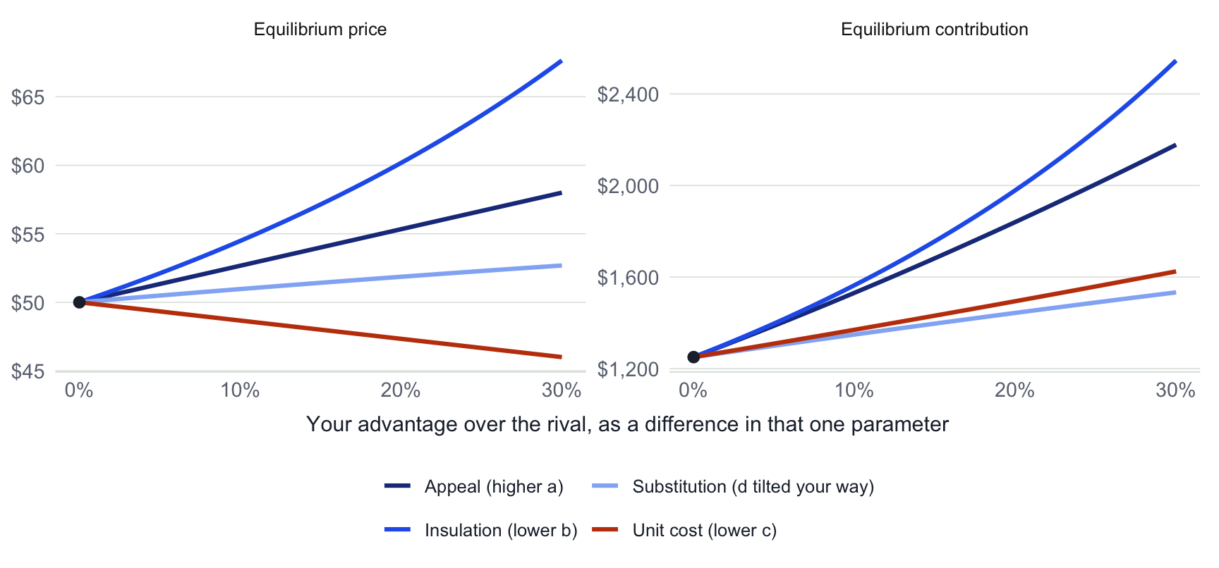
Read the right-hand panel first, because the ranking is the surprise. A thirty percent edge in insulation buys about three and a half times the contribution that the same edge in unit cost does, and the insulation line is still accelerating when the others have gone nearly straight. Low \(\mathsf{b}\) compounds: customers who do not leave when you raise price let you raise it again. Nothing else in the figure compounds.
Substitution is the weakest of the four, which is worth knowing before you spend a year engineering switching costs. Tilting the flow your way helps, and it helps about a fifth as much as making your own customers stickier by the same proportion. It is the only lever in the figure that a cost advantage beats.
Then the left-hand panel, where the cost line goes the wrong way. A cost advantage lowers your equilibrium price. You pass part of the saving through, because your best response to your own lower cost is to charge less, and the profit arrives as volume rather than as a fatter price tag. Every founder who has said we can make it cheaper, so we can charge the same and pocket the difference has this backwards; the equilibrium will not let you.
Some, never all, and the fraction is not yours to choose. Differentiating the equilibrium gives the pass-through rate
\[ \frac{\partial \mathsf{p_i}}{\partial \mathsf{c_i}} \;=\; \frac{1}{2}\left(1 - \frac{\mathsf{d_i d_j}}{4\,\mathsf{b_i b_j}}\right)^{-1} \]
which sits at exactly one half when the two firms are unconnected, and climbs toward one as the coupling between them tightens. Two isolated firms each keep half of any cost saving as margin. Two tightly coupled ones keep almost none of it, because a cost advantage you pass into price pulls your rival’s best response down, which pulls yours down again.
Whether your margin widens at all turns on the same quantity. It widens when \(\mathsf{d_i d_j < 2\,b_i b_j}\) and shrinks when the inequality runs the other way, so the sign of the thing depends on a product of four parameters, only two of which are yours. In practice it will widen: shrinking requires cross-price effects so strong that one firm raising its price grows the whole market, which is a sign the demand system was estimated badly rather than a market anyone has met. The useful part is not the sign. It is that how much of a cost advantage survives to your bottom line is set by how tightly you are coupled to a rival, and you can compute it from four numbers you already have.
One parameter is missing from the figure, and its absence is the point. Fixed cost \(\mathsf{f}\) does not appear in the equilibrium at all; it is subtracted after both prices are set, so it cannot move a best response and cannot make you a better competitor. What it does is decide whether the contribution you just computed is enough. A rival with lower \(\mathsf{f}\) does not out-compete you — they outlast you, at an equilibrium you both reached together. That makes \(\mathsf{f}\) a survival threshold rather than an advantage, which is the same reading scale and population gave it when it set the penetration you had to reach.
The clearest way to see all of this at once is a case where the intuition was wrong.
A Campus Case
When the franchise should have won
Smart Cookie opened near a university campus selling one thing well: ice cream sandwiches made from gourmet cookies. It did that for several years, successfully, until a franchise sandwich shop across the way, Hogi Yogi, introduced a nearly identical ice cream sandwich at a lower price.
The expectation was straightforward. The franchise had scale, a lower cost structure, and an established brand. It should have taken the market.
It did not. The lines at Smart Cookie stayed long.
To find out why, we surveyed their customers, and estimated a differentiated demand system from what those customers said they would buy at what prices:
\[\mathsf{q_{sc} = -0.70 - 2.16\,p_{sc} + 5.57\,p_{hy}}\] \[\mathsf{q_{hy} = \phantom{-}4.57 - 3.50\,p_{hy} + 0.55\,p_{sc}}\]
with variable costs of $0.75 for Smart Cookie and $0.50 for Hogi Yogi.
Read the asymmetries before reading the outcome. Hogi Yogi does have the cost advantage, by twenty-five cents a unit. But its customers are more price-sensitive, not less: 3.50 against Smart Cookie’s 2.16. And the switching is wildly lopsided. When Hogi Yogi raises price, 5.57 units of demand move to Smart Cookie. When Smart Cookie raises price, 0.55 move the other way — a tenth as much.
Solving for where the two best responses cross gives prices of $1.53 and $1.02, and monthly contribution per customer of $1.33 and $0.96. The predicted prices came within pennies of what the two shops were actually charging.
So the franchise’s cost advantage was real and it was not enough. It was outweighed by two demand-side asymmetries that nobody had thought to measure, and that no amount of operational excellence would have revealed.
That case is small enough to see all the way through, and the same structure appears at any scale. Gasmi, Laffont and Vuong estimated a demand system for cola concentrate over the years 1968 to 1986 (Gasmi et al. 1992). Read at the averages of their sample, their parameters put Coca-Cola’s appeal at 63.4 against Pepsi’s 49.5, its own-price sensitivity at 3.98 against 5.48, and its substitution gain at 2.25 against Pepsi’s 1.40 — while Pepsi holds the cost advantage, $3.96 against $4.96. Equilibrium prices come out near $12.74 and $8.12, with Coke earning roughly two and a half times the contribution. The same check applies as it did to the ice cream, and it survives it: across those years the two firms were actually charging $12.96 and $8.16.
Twice, at wildly different scales, the firm with the cost advantage lost. That is not a coincidence and it is not a rule that cost never matters. It is what happens when a cost advantage of one size meets demand-side insulation of a larger one.
One thing to notice about the Smart Cookie estimates
The intercept for Smart Cookie is negative, which read literally says that at a price of zero, demand is below nothing. That is not a finding about ice cream. It is a straight line being extended past the prices anyone was ever charged, which is the caution from estimating demand arriving in a real dataset.
It does no damage here because the equilibrium sits inside the range where the data actually lives. It would do damage the moment anyone used this system to ask about a price of fifty cents. A fitted parameter is trustworthy over the prices you observed and is a guess everywhere else, and that remains true when the fit is excellent.
What Makes an Advantage Durable
Having an advantage and keeping it are different questions, and the second one sorts the four parameters differently from the first.
Size comes first. When the asymmetry is small the equilibrium barely moves — prices differ by pennies, profits differ marginally, and a competitor’s ordinary response erases it. A modest price cut, a small product change, a routine cost improvement. An advantage that a rival can undo in a quarter was a head start rather than a position.
Then imitability, and here the ranking inverts.
Cost advantages are usually the most visible and the most copyable. Operations improve, technology spreads, suppliers sell to everyone, and whatever made you cheaper is generally legible to anyone who looks hard.
Usually, and not always, and the exceptions are worth knowing because they point at which kind of cost advantage to build. A cost advantage that comes from what an organization has learned behaves very differently from one that comes from what it bought, and it behaves less comfortably than the phrase “learning curve” suggests. Studying wartime and industrial production, Argote et al. (1990) found that knowledge acquired through production depreciates rapidly, so cumulative output badly overstates how much of it a firm still holds — and that once a firm is producing, it does not appear to benefit from what other firms have learned. Learning is harder to keep and harder to steal at the same time. Semiconductor plants that invested in the human capital of their operators moved down the learning curve faster and held the resulting cost advantage, and it did not transfer to rivals even when the operators themselves did, because much of what those people knew was specific to that plant and did not travel with them (Hatch and Dyer 2004). Toyota’s production advantages were similarly slow to reach its American rivals even where the same suppliers were building parts for both, in the same buildings, because the advantage lived in the relationships rather than in the equipment (Dyer and Hatch 2006).
Slow is not permanent. The American manufacturers largely closed that gap in the end. That is the useful part rather than a qualification of it: a cost advantage built out of what people and networks know can outlast the patience of the firms trying to copy it, and it is a different asset from a cost advantage built out of a purchase order.
Demand-side insulation is harder to see and harder to erode. Low \(\mathsf{b}\) means customers who do not leave when you raise price, and that comes from things a competitor cannot buy in a quarter: trust built over years, a product genuinely suited to a specific group, switching costs, habit, identity. Smart Cookie’s advantage was of this kind, which is why a franchise with a cost edge could not dislodge it.
Substitution asymmetry sits between them. Being the firm customers defect to rather than from is genuine insulation, and it is more fragile than low price sensitivity because it depends partly on your rival’s choices as well as your own.
So the diagnostic. An advantage is durable when the asymmetry is large, when it sits in price sensitivity or substitution rather than only in cost, and when its underlying cause is something a competitor would find expensive and slow to replicate. It is fragile when parameters are nearly symmetric, when customers move quickly on price, and when the difference between you comes down to something a well-run rival could copy by Christmas.
Scale Is Not Advantage
One correction to make before the entry question, because it is the most common way this analysis gets misused.
In differentiated Bertrand competition, the rival’s size does not appear anywhere in the equilibrium. Only demand parameters and costs do. A large incumbent serving a broad population does not, by being large, force your price down. What moves your price is how sensitive your customers are, how readily they switch, and what it costs you to serve them.
That has a consequence entrepreneurs routinely get backwards. A large addressable market is not a structural advantage; it is a multiplier on whatever structure you have. Multiply a fragile position by a big market and you get a bigger fragile position. And a small, well-insulated segment can sustain high prices and durable profit indefinitely, which is why so many good businesses look too small to be interesting.
The discipline that follows is to evaluate advantage locally before extrapolating it. Define the population you can actually serve, estimate demand inside it, compute the equilibrium there, and only then ask about expansion. Doing it the other way around produces a number that is large and means nothing.
There are real exceptions, and they are specific rather than general: when capacity binds, when network effects make demand depend on how many others have already bought, or when the same two firms meet each other across several markets at once. Absent one of those, scale multiplies structure without creating it.
Entry Is a Forecast About Equilibrium
Now the decision this part of the book has been building toward.
When you consider entering a market that already has someone in it, the question is not whether demand exists. Demand almost always exists; that is usually what attracted you. The question is what profit you will earn after the incumbent has responded, which is to say at the equilibrium the two of you will produce together.
That reframing makes entry barriers concrete. A barrier is usually described as a wall — capital requirements, patents, regulation, brand. Analytically it is simpler and less romantic than that:
An entry barrier is structural asymmetry large enough to make the entrant’s equilibrium profit negative.
Nothing keeps you out. You are perfectly free to enter, and the arithmetic says you will lose money when you do.
Which tells you what to do about it, and it is not to try harder. If the parameters are against you where the incumbent is strong, find the place where they are not. That is the pattern Bryce and Dyer (2007) found across entrants into the most profitable American industries of the 1990s: the ones that got in did not attack head-on, but leveraged assets they already had, rearranged the value chain, or started in a niche the incumbent was not defending. Their cola example is worth holding next to the numbers above. Virgin Drinks went straight at mainstream retail in 1998, against the appeal and distribution the incumbents were strongest in, and never took one percent of the market. Red Bull started the year before in bars and nightclubs, a segment where the parameters were its own, and by 2005 held roughly two thirds of a market that had not previously existed. In the language of this chapter, the entrant does not beat the incumbent’s parameters. It goes somewhere the parameters are different. If the incumbent has higher appeal, lower price sensitivity, favorable substitution, or lower cost, and the gap is wide enough, your equilibrium profit is zero or below before you sign anything. That is a parameter configuration rather than a slogan, and you can compute it in advance.
It also explains what deterrence actually is. An incumbent who invests in visible capacity, signals low cost, or raises switching costs is not frightening you. They are changing your forecast, by making it credible that post-entry competition will be severe enough that your equilibrium profit is negative. Deterrence works when the structural asymmetry is real, and it works nearly as well when a potential entrant merely believes it is.
Why Entry Happens Anyway
Which raises an obvious problem. If barriers are structural and computable, why does entry into hopeless markets happen constantly?
Because forecasting an equilibrium is cognitively demanding, and the alternative is available and feels like confidence. Doing it properly means anticipating the post-entry price, believing the incumbent’s advantages are real, and trusting arithmetic over enthusiasm at exactly the moment enthusiasm is highest. The failure modes are predictable: overestimate your appeal, underestimate how readily customers substitute, wave away a cost disadvantage, and above all assume the incumbent will stand still.
That last one is the load-bearing error, and it is the one this whole part of the book exists to remove.
There is evidence on what that error costs, and it is stranger than a ranking of who does better.
That firms act on a representation of their competitive situation rather than on the situation itself is an old finding, and a well-evidenced one.1 What is newer is the question of whose representation does the work.
Simulating entry into new and uncertain markets, where each firm holds some representation of the market and of its rival, the value of a representation turns out to be relational rather than intrinsic.2
Sit with that for a moment. In a market with one competitor, how they see the situation can matter more to your outcome than how you see it. You can be right about demand and still be wrecked by a rival whose blindness to rivalry makes them reckless, or handed the market by one whose caution concedes it.
The exposure is not evenly spread, which is where the practical reading comes in. It is concentrated among firms that are blind to rivalry. A representation that combines awareness of the rival with the flexibility to wait largely insures its holder against the other firm’s mind — and that combination is precisely what this part of the book has been building. Represent the competition as something that responds, estimate the parameters, compute where the market settles, and keep your options open until you have.
There is one more result worth carrying, because it rhymes with everything else in this part. Identically matched representations underperform. Two firms thinking about the market in exactly the same way do worse than two thinking differently, which puts a premium on cognitive differentiation between rivals. Being distinctive turns out to matter one level further up than we have been treating it: not only in what you sell, but in how you see.
Ask yourself — which parameter is yours, and how long do you keep it?
Name your closest competitor and write down four comparisons. Is your appeal higher? Are your customers less sensitive to your price? Do you gain more from their price rise than they gain from yours? Is your unit cost lower?
If the honest answer to all four is no, you do not have a competitive advantage. That is not a verdict on the venture, and it is a fact worth knowing before you commit.
If one or two are yes, ask the harder question about each: how large, and how long. A five percent edge in unit cost that a competent rival could match this year is not the same asset as customers who would stay with you through a ten percent price rise. One of those shows up in an equilibrium and stays there; the other shows up and leaves.
Then say plainly which of your advantages you would still have in three years if your rival were paying attention. The ones that survive that sentence are the ones your decision can rest on.
The move: Advantage is a measurable asymmetry in four parameters, not a story about your product. Cost advantages are the easiest to see and the easiest to copy; the ones that last are the ones that make your customers slow to leave.
This is as far as price alone will take the argument. Both firms have been choosing one number, simultaneously, forever, with nothing else to decide and no way to move first. Real rivals advertise, add capacity, launch, wait, and commit to things specifically so the other firm has to respond. Those choices have a logic of their own, and price is only the simplest thing two firms ever fight about.
Studying Scottish knitwear manufacturers, Porac et al. (1989) found that firms did not compete against everyone making knitwear. They competed against the handful they believed were their rivals, and those beliefs were shared across the group, stable, and reinforced by the very structure they described — the industry both shaping managers’ models of it and being shaped by them. The follow-up traced how that shared model held together and where its boundaries actually ran (Porac et al. 1995). The lesson worth carrying is that your rival set is a mental object before it is an economic one, which is why naming the wrong rival is a real risk rather than a hypothetical one. What you attend to determines your own decisions, and it also determines how exposed you are to whatever the other firm happens to believe. Across most of the environments simulated, the rival’s representation explained more of the variation in a firm’s performance than that firm’s own representation did.↩︎